5. Bayesian Hierarchical Joint Modeling for Historical Data Borrowing

The purpose of this document is to show a minimal workflow for Bayesian hierarchical joint modeling for historical data borrowing using the jmpost package.

Setup and load data

Here we execute the R code from the setup and data preparation chapter, see the full code here.

Descriptive analysis of the current study data

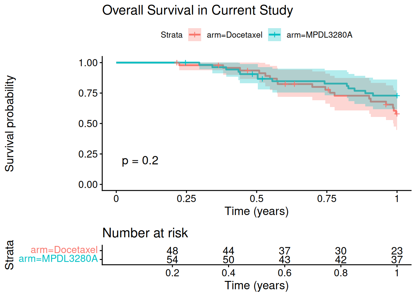
Let’s have a quick look at the (artificially reduced to maximum 1 year follow-up) current study data, in order to illustrate the typical situation where we have immature OS data:

library(survival)

Attaching package: 'survival'

The following object is masked from 'package:brms':

    kidney

library(survminer)

Loading required package: ggpubr

Attaching package: 'survminer'

The following object is masked from 'package:survival':

    myeloma

# Overall Survival KM plot
fit_os_current <- survfit(Surv(os_time, os_event) ~ arm, data = current_os_data)

ggsurvplot(
    fit_os_current,
    data = current_os_data,
    risk.table = TRUE,
    pval = TRUE,
    conf.int = TRUE,
    xlab = "Time (years)",
    title = "Overall Survival in Current Study"
)

Warning: Using `size` aesthetic for lines was deprecated in ggplot2 3.4.0.
ℹ Please use `linewidth` instead.
ℹ The deprecated feature was likely used in the ggpubr package.
  Please report the issue at <https://github.com/kassambara/ggpubr/issues>.

Ignoring unknown labels:
• colour : "Strata"

So no matter which model we might fit to this data, we will not be able to trust it to estimate the hazard ratio reliably.

Check compatibility of historical and current data

Just to mention that we would need to double check the compatibility of historical and current clinical trial design (including patient populations, endpoints, assessment schedules, etc.) and data distributions before applying any kind of historical data borrowing technique.

In our dummy example here, this is fulfilled by construction.

Fitting the joint model only to the historical data

The first step is to fit the joint model only to the historical data. In reality, this also includes model selection in order to determine:

• choice of parametric baseline survival model (log-logistic, Weibull, etc.?)
• selection of baseline covariates
• choice of the TGI metric to correlate with the survival model, i.e. the link function (SLD, tumor growth rate, time to tumor regrowth, etc.?)

We have discussed model comparison and selection in session 3 here, so we will skip this step here and directly fit a joint model to the historical data only.

historical_subj_df <- historical_os_data |>
    select(study, id, arm)
historical_subj_data <- DataSubject(
    data = historical_subj_df,
    subject = "id",
    arm = "arm",
    study = "study"
)

historical_long_df <- historical_tumor_data |>
    select(id, year, sld)
historical_long_data <- DataLongitudinal(
    data = historical_long_df,
    formula = sld ~ year
)

historical_surv_data <- DataSurvival(
    data = historical_os_data,
    formula = Surv(os_time, os_event) ~ ecog + age + race + sex
)

historical_joint_data <- DataJoint(
    subject = historical_subj_data,
    longitudinal = historical_long_data,
    survival = historical_surv_data
)

historical_joint_mod <- JointModel(
    longitudinal = LongitudinalSteinFojo(
        mu_bsld = prior_normal(log(65), 1),
        mu_ks = prior_normal(log(0.52), 1),
        mu_kg = prior_normal(log(1.04), 1),
        omega_bsld = prior_normal(0, 3) |> set_limits(0, Inf),
        omega_ks = prior_normal(0, 3) |> set_limits(0, Inf),
        omega_kg = prior_normal(0, 3) |> set_limits(0, Inf),
        sigma = prior_normal(0, 3) |> set_limits(0, Inf)
    ),
    survival = SurvivalWeibullPH(
        lambda = prior_gamma(0.7, 1),
        gamma = prior_gamma(1.5, 1),
        beta = prior_normal(0, 20)
    ),
    link = linkGrowth(
        prior = prior_normal(0, 20)
    )
)

options("jmpost.prior_shrinkage" = 0.999)

save_file <- here("session-bhm/histmod1.rds")
if (file.exists(save_file)) {
    historical_joint_results <- readRDS(save_file)
} else {
    historical_joint_results <- sampleStanModel(
        historical_joint_mod,
        data = historical_joint_data,
        iter_sampling = ITER,
        iter_warmup = WARMUP,
        chains = CHAINS,
        parallel_chains = CHAINS,
        thin = CHAINS,
        seed = BAYES.SEED,
        refresh = REFRESH
    )
    saveObject(historical_joint_results, file = save_file)
}

Let’s have a look at the results:

vars <- c(
    "lm_sf_mu_bsld",
    "lm_sf_mu_ks",
    "lm_sf_mu_kg",
    "lm_sf_sigma",
    "lm_sf_omega_bsld",
    "lm_sf_omega_ks",
    "lm_sf_omega_kg",
    "beta_os_cov",
    "sm_weibull_ph_gamma",
    "sm_weibull_ph_lambda",
    "link_growth"
)

mcmc_historical_joint_results <- cmdstanr::as.CmdStanMCMC(historical_joint_results)

mcmc_historical_summary <- mcmc_historical_joint_results$summary(vars)

print(mcmc_historical_summary, n = 30)

# A tibble: 19 × 10
   variable         mean   median      sd     mad      q5     q95  rhat ess_bulk
   <chr>           <dbl>    <dbl>   <dbl>   <dbl>   <dbl>   <dbl> <dbl>    <dbl>
 1 lm_sf_mu_bs…  3.75     3.76    0.0519  0.0510   3.67    3.84   1.01      208.
 2 lm_sf_mu_ks…  0.0560   0.0818  0.257   0.246   -0.399   0.440  1.00      775.
 3 lm_sf_mu_ks… -0.913   -0.865   0.388   0.385   -1.60   -0.353  1.00      683.
 4 lm_sf_mu_kg… -0.496   -0.491   0.126   0.120   -0.699  -0.290  0.999     732.
 5 lm_sf_mu_kg… -0.782   -0.773   0.198   0.189   -1.12   -0.473  1.00      614.
 6 lm_sf_sigma   0.121    0.120   0.00479 0.00459  0.113   0.129  1.00      951.
 7 lm_sf_omega…  0.493    0.490   0.0359  0.0340   0.438   0.557  1.00      590.
 8 lm_sf_omega…  0.913    0.891   0.195   0.181    0.640   1.27   1.00      850.
 9 lm_sf_omega…  1.26     1.21    0.302   0.281    0.837   1.80   1.00      649.
10 lm_sf_omega…  0.458    0.453   0.0903  0.0907   0.324   0.607  1.00      775.
11 lm_sf_omega…  0.990    0.975   0.133   0.131    0.796   1.24   1.00      766.
12 beta_os_cov…  1.17     1.17    0.380   0.364    0.518   1.79   1.00      895.
13 beta_os_cov…  0.00931  0.00952 0.0153  0.0155  -0.0150  0.0342 1.000     987.
14 beta_os_cov…  0.942    0.940   0.653   0.628   -0.153   2.00   1.00     1015.
15 beta_os_cov…  0.165    0.157   0.374   0.379   -0.440   0.778  1.00     1051.
16 beta_os_cov…  0.246    0.239   0.331   0.325   -0.272   0.789  1.00     1049.
17 sm_weibull_…  1.70     1.70    0.212   0.203    1.35    2.06   1.00      980.
18 sm_weibull_…  0.151    0.0983  0.163   0.0881   0.0162  0.460  0.998    1001.
19 link_growth   0.988    0.985   0.375   0.370    0.377   1.59   1.00      796.
# ℹ 1 more variable: ess_tail <dbl>

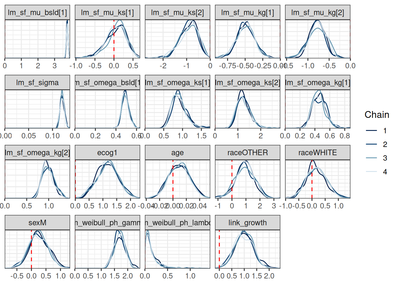
Let’s also look at the covariate effect estimates again:

os_cov_name_mapping <- function(surv_data) {
    surv_data_design <- as_stan_list(surv_data)$os_cov_design
    os_cov_names <- colnames(surv_data_design)
    old_coef_names <- as.character(glue::glue("beta_os_cov[{seq_along(os_cov_names)}]"))
    setNames(old_coef_names, os_cov_names)
}
os_cov_renaming <- os_cov_name_mapping(historical_surv_data)

draws_historical_joint_results <- mcmc_historical_joint_results$draws(vars)
draws_historical_joint_results <- do.call(
    rename_variables,
    c(list(draws_historical_joint_results), os_cov_renaming)
)
mcmc_dens_overlay(draws_historical_joint_results) +
    geom_vline(xintercept = 0, linetype = "dashed", color = "red")

Pool historical and current data

Now we pool the historical and the current data for the hierarchical joint modeling step:

pooled_os_data <- bind_rows(
    historical_os_data,
    current_os_data
)
pooled_tumor_data <- bind_rows(
    historical_tumor_data,
    current_tumor_data
)
pooled_subj_df <- pooled_os_data |>
    select(study, id, arm)

pooled_subj_data <- DataSubject(
    data = pooled_subj_df,
    subject = "id",
    arm = "arm",
    study = "study"
)

pooled_long_df <- pooled_tumor_data |>
    select(id, year, sld)
pooled_long_data <- DataLongitudinal(
    data = pooled_long_df,
    formula = sld ~ year
)

pooled_surv_data <- DataSurvival(
    data = pooled_os_data,
    formula = Surv(os_time, os_event) ~ ecog + age + race + sex
)
pooled_joint_data <- DataJoint(
    subject = pooled_subj_data,
    longitudinal = pooled_long_data,
    survival = pooled_surv_data
)

So now we have pooled our 101 historical and 102 current patients into a single data set with 203 patients.

Fit the Bayesian hierarchical joint model

Now we can fit the Bayesian hierarchical joint model to the pooled data set, borrowing information from the historical data to inform the current data analysis.

Note that we use the same model specification historical_joint_mod as for the historical data only model fit above. The reason is that the LongitudinalSteinFojo class already accounts for hierarchical modeling, see the statistical specification here.

save_file <- here("session-bhm/pooledmod1.rds")
if (file.exists(save_file)) {
    pooled_joint_results <- readRDS(save_file)
} else {
    pooled_joint_results <- sampleStanModel(
        historical_joint_mod,
        data = pooled_joint_data,
        iter_sampling = ITER,
        iter_warmup = WARMUP,
        chains = CHAINS,
        parallel_chains = CHAINS,
        thin = CHAINS,
        seed = BAYES.SEED,
        refresh = REFRESH
    )
    saveObject(pooled_joint_results, file = save_file)
}

Let’s first check again if the MCMC sampling went fine:

mcmc_pooled_joint_results <- cmdstanr::as.CmdStanMCMC(pooled_joint_results)

mcmc_pooled_summary <- mcmc_pooled_joint_results$summary(vars)

print(mcmc_pooled_summary, n = 30)

# A tibble: 21 × 10
   variable         mean   median      sd     mad      q5     q95  rhat ess_bulk
   <chr>           <dbl>    <dbl>   <dbl>   <dbl>   <dbl>   <dbl> <dbl>    <dbl>
 1 lm_sf_mu_bs…  3.75     3.75    0.0578  0.0577   3.65    3.84   1.02      247.
 2 lm_sf_mu_bs…  3.76     3.76    0.0490  0.0479   3.67    3.84   1.02      140.
 3 lm_sf_mu_ks… -0.0438  -0.0213  0.228   0.215   -0.454   0.301  1.01      582.
 4 lm_sf_mu_ks… -1.04    -1.01    0.316   0.305   -1.58   -0.581  1.00      618.
 5 lm_sf_mu_kg… -0.587   -0.581   0.129   0.133   -0.807  -0.386  1.01      510.
 6 lm_sf_mu_kg… -0.873   -0.875   0.141   0.144   -1.10   -0.646  1.00      519.
 7 lm_sf_sigma   0.129    0.129   0.00366 0.00361  0.123   0.136  1.00      719.
 8 lm_sf_omega…  0.573    0.569   0.0408  0.0416   0.514   0.644  1.00      393.
 9 lm_sf_omega…  0.492    0.487   0.0370  0.0360   0.436   0.555  1.00      386.
10 lm_sf_omega…  0.956    0.945   0.165   0.163    0.720   1.24   1.01      530.
11 lm_sf_omega…  1.35     1.32    0.248   0.227    1.02    1.79   1.01      512.
12 lm_sf_omega…  0.682    0.675   0.0831  0.0826   0.557   0.827  1.00      884.
13 lm_sf_omega…  0.961    0.950   0.101   0.0995   0.810   1.14   1.00      595.
14 beta_os_cov…  1.16     1.15    0.285   0.285    0.687   1.62   1.00      934.
15 beta_os_cov…  0.00105  0.00131 0.0118  0.0114  -0.0190  0.0202 0.999     965.
16 beta_os_cov…  1.16     1.16    0.508   0.489    0.338   1.97   1.00     1003.
17 beta_os_cov…  0.171    0.167   0.299   0.301   -0.303   0.666  1.00      897.
18 beta_os_cov…  0.263    0.262   0.262   0.268   -0.159   0.708  1.00      834.
19 sm_weibull_…  1.92     1.91    0.201   0.195    1.60    2.25   0.998     930.
20 sm_weibull_…  0.255    0.191   0.212   0.137    0.0551  0.699  1.00     1002.
21 link_growth   1.18     1.18    0.281   0.276    0.708   1.64   0.999     816.
# ℹ 1 more variable: ess_tail <dbl>

Indeed all rhat values are close to 1 indicating convergence.

Investigating the parameter estimates

We can see that now we have more model parameters, let’s see which are additional compared to the historical data only model:

pooled_param_names <- mcmc_pooled_summary$variable
historical_param_names <- mcmc_historical_summary$variable
new_params <- setdiff(pooled_param_names, historical_param_names)
new_params

[1] "lm_sf_mu_bsld[2]"    "lm_sf_omega_bsld[2]"

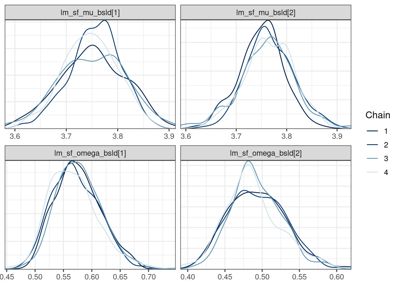
We see that the additional parameters correspond to the baseline value, which is supposed to differ between studies: both the mean mu parameter and the standard deviation omega parameter gain an additional second dimension here with the addition of the second study.

Let’s look at the estimates of these new parameters and compare them between the studies:

baseline_vars <- c("lm_sf_mu_bsld", "lm_sf_omega_bsld")
baseline_pooled_joint_results <- mcmc_pooled_joint_results$draws(baseline_vars)

mcmc_dens_overlay(baseline_pooled_joint_results)

library(posterior)

# Convert draws to rvars for easier manipulation
baseline_rvars <- as_draws_rvars(baseline_pooled_joint_results)

mu_diff <- baseline_rvars$lm_sf_mu_bsld[1] - baseline_rvars$lm_sf_mu_bsld[2]
summary(mu_diff)

# A tibble: 1 × 10
  variable     mean   median     sd    mad     q5   q95  rhat ess_bulk ess_tail
  <chr>       <dbl>    <dbl>  <dbl>  <dbl>  <dbl> <dbl> <dbl>    <dbl>    <dbl>
1 mu_diff  -0.00927 -0.00803 0.0742 0.0752 -0.134 0.112  1.00     228.     356.

omega_diff <- baseline_rvars$lm_sf_omega_bsld[1] - baseline_rvars$lm_sf_omega_bsld[2]
summary(omega_diff)

# A tibble: 1 × 10
  variable     mean median     sd    mad       q5   q95  rhat ess_bulk ess_tail
  <chr>       <dbl>  <dbl>  <dbl>  <dbl>    <dbl> <dbl> <dbl>    <dbl>    <dbl>
1 omega_diff 0.0812 0.0803 0.0553 0.0548 -0.00772 0.172  1.00     351.     601.

As expected we don’t see a big difference in the baseline SLD between the historical and current study, neither in the mean nor in the standard deviation.

Goodness of fit

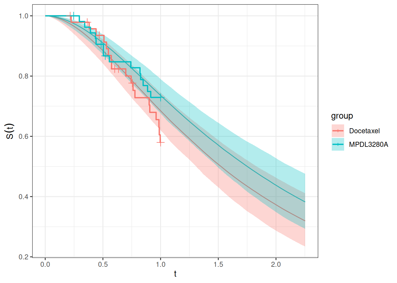
Let’s check the goodness of fit to our current study data:

current_subj_df <- current_os_data |>
    select(study, id, arm)

time_grid <- seq(from = 0, to = max(pooled_os_data$os_time), length = 100)
current_os_surv_group_grid <- GridGrouped(
    times = time_grid,
    groups = with(
        current_subj_df,
        split(as.character(id), arm)
    )
)
current_os_surv_pred <- SurvivalQuantities(
    object = pooled_joint_results,
    grid = current_os_surv_group_grid,
    type = "surv"
)

autoplot(current_os_surv_pred, add_km = TRUE, add_wrap = FALSE)

So the fit looks satisfactory, considering that the current data are quite immature.

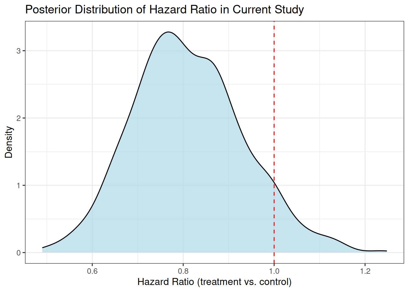
Posterior distribution of the hazard ratio

Now let’s look at the posterior distribution of the hazard ratio between the two treatment arms in the current study. We do this as follows:

• For a given MCMC sample \(i\):
  • Sample predicted survival times for the current study subjects which are still being followed up
  • Fit a Cox proportional hazards regression model
  • Extract the hazard ratio estimate
• Repeat for all MCMC samples to get the posterior distribution of the hazard ratio

This is the same algorithm we used in the session 4 here.

In this example we assume for simplicity:

• no additional patients will be enrolled, i.e. we don’t need to add new patients to the data set
• all currently censored patients will be followed up until event occurs

Therefore we can directly jump into the sampling step as described here:

# Determine for which patients we want to sample the individual survival times.
pt_to_sample <- pooled_os_data |>
    filter(study == "current" & os_event == 0)
pt_to_sample_ids <- pt_to_sample$id

# Obtain the survival function samples (for all patients here).
length_time_grid <- 100
time_grid_end <- round(max(pooled_os_data$os_time) + 10, 1)
time_grid <- seq(0, time_grid_end, length = length_time_grid)

save_file <- here("session-bhm/bhm1_surv_samples.rds")
if (file.exists(save_file)) {
    os_surv_samples <- readRDS(save_file)
} else {
    os_surv_samples <- SurvivalQuantities(
        object = pooled_joint_results,
        grid = GridFixed(times = time_grid),
        type = "surv"
    )
    saveRDS(os_surv_samples, file = save_file)
}

qs <- os_surv_samples@quantities
include_qs <- qs@groups %in% pt_to_sample_ids

qs_samples <- qs@quantities[, include_qs]
qs_times <- qs@times[include_qs]
qs_groups <- qs@groups[include_qs]

surv_values_samples <- matrix(
    qs_samples,
    nrow = ITER * length(pt_to_sample_ids),
    ncol = length_time_grid
)

surv_values_pt_ids <- rep(
    head(qs_groups, length(pt_to_sample_ids)),
    each = ITER
)

censoring_times <- pt_to_sample$os_time[match(
    surv_values_pt_ids,
    pt_to_sample_ids
)]

library(Rcpp)

# Use Rcpp function for single patient, single sample.
sourceCpp(here("session-pts/conditional_sampling.cpp"))

cond_surv_time_samples <- sample_conditional_survival_times(
    time_grid = time_grid,
    surv_values = surv_values_samples,
    censoring_times = censoring_times
)

os_cond_samples <- matrix(
    cond_surv_time_samples$t_results,
    nrow = ITER,
    ncol = length(pt_to_sample_ids),
    dimnames = list(seq_len(ITER), head(qs_groups, length(pt_to_sample_ids)))
)

The next step is again to create the complete OS data sets. Here we just use the current data set and replace the censored times with the sampled times above:

os_rows_to_replace <- match(
    pt_to_sample_ids,
    current_os_data$id
)

os_cond_samples_cols <- match(
    pt_to_sample_ids,
    colnames(os_cond_samples)
)

os_data_samples <- lapply(1:ITER, function(i) {
    # Create a copy of the original OS data
    os_data_sample <- current_os_data[, c("id", "arm", "os_time", "os_event", "race", "sex", "ecog", "age")]

    # Add the sampled OS times for the patients who are still being followed up.
    os_data_sample$os_time[os_rows_to_replace] <- os_cond_samples[
        i,
        os_cond_samples_cols
    ]

    # Set the OS event to TRUE for those patients, because we assume they have an event now.
    os_data_sample$os_event[os_rows_to_replace] <- TRUE

    os_data_sample
})

Now we can fit a Cox proportional hazards regression model to each of the completed data sets and extract the hazard ratio estimates:

hr_est_fun <- function(df) {
    cox_mod <- coxph(Surv(os_time, os_event) ~ arm,
        data = df
    )
    exp(unname(coef(cox_mod)))
}

We can try on one data set first:

hr_est_fun(os_data_samples[[1]])

[1] 0.8503437

Now we can apply this to all data sets:

hr_estimates <- sapply(os_data_samples, hr_est_fun)

We can visualize this:

library(ggplot2)
hr_df <- data.frame(hr = hr_estimates)
ggplot(hr_df, aes(x = hr)) +
    geom_density(fill = "lightblue", alpha = 0.7) +
    geom_vline(xintercept = 1, linetype = "dashed", color = "red") +
    xlab("Hazard Ratio (treatment vs. control)") +
    ylab("Density") +
    ggtitle("Posterior Distribution of Hazard Ratio in Current Study")

Probability of success

Let’s assume the minimal detectable difference, i.e. the hazard ratio that we would consider clinically relevant, is 0.75. Then our probability of success is given by the posterior probability that the hazard ratio is below 0.75:

mean(hr_estimates < 0.75)

[1] 0.326