---
title: "1. TGI model minimal workflow with `brms`"
author:
- Daniel Sabanés Bové
- Francois Mercier
date: last-modified
editor_options:
chunk_output_type: inline
format:
html:
code-fold: show
html-math-method: mathjax
cache: true
---
The purpose of this document is to show a minimal workflow for fitting a TGI model using the `brms` package.
## Setup and load data
{{< include _setup_and_load.qmd >}}
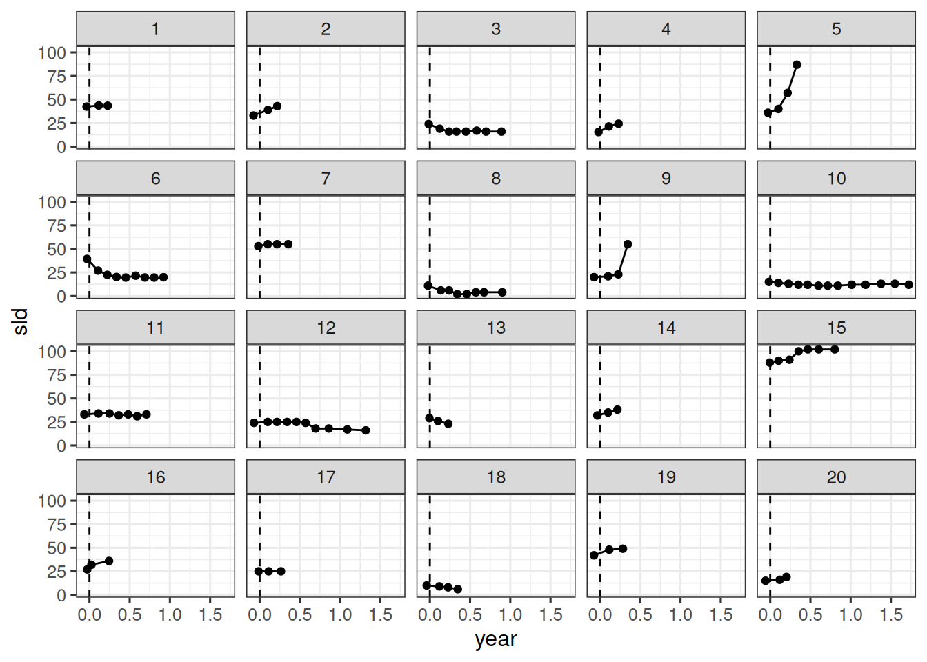
{{< include _load_data.qmd >}}
## Stein-Fojo model
We start from the Stein-Fojo model as shown in the slides:
$$
y^{*}(t_{ij}) = \psi_{b_{0}i} \{\exp(- \psi_{k_{s}i} \cdot t_{ij}) + \exp(\psi_{k_{g}i} \cdot t_{ij}) - 1\}
$$
### Mean
We will make one more tweak here. If the time $t$ is negative, i.e. the treatment has not started yet, then it is reasonable to assume that the tumor cannot shrink yet. Therefore, the final model for the mean SLD is:
$$
y^{*}(t_{ij}) =
\begin{cases}
\psi_{b_{0}i} \exp(\psi_{k_{g}i} \cdot t_{ij}) & \text{if } t_{ij} < 0 \\
\psi_{b_{0}i} \{\exp(-\psi_{k_{s}i} \cdot t_{ij}) + \exp(\psi_{k_{g}i} \cdot t_{ij}) - 1\} & \text{if } t_{ij} \geq 0
\end{cases}
$$
### Likelihood
For the likelihood given the mean SLD $y^{*}$, we will assume a normal distribution with a constant coefficient of variation $\tau$:
$$
y(t_{ij}) \sim \text{N}(y^{*}(t_{ij}), y^{*}(t_{ij})\tau)
$$
Note that for consistency with the `brms` and `Stan` convention, here we denote the standard deviation as the second parameter of the normal distribution. So in this case, the variance would be $(y^{*}(t_{ij})\tau)^2$.
This can also be written as:
$$
y(t_{ij}) = (1 + \epsilon_{ij}) \cdot y^{*}(t_{ij})
$$
where $\epsilon_{ij} \sim \text{N}(0, \tau)$.
Note that also the additive model is a possible choice, where
$$
y(t_{ij}) = y^{*}(t_{ij}) + \epsilon_{ij}
$$
such that the error does not depend on the scale of the SLD any longer.
### Random effects
Next, we define the distributions of the random effects $\psi_{b_{0}i}$, $\psi_{k_{s}i}$, $\psi_{k_{g}i}$, for $i = 1, \dotsc, n$:
$$
\begin{align*}
\psi_{b_{0}i} &\sim \text{LogNormal}(\mu_{b_{0}}, \omega_{0}) \\
\psi_{k_{s}i} &\sim \text{LogNormal}(\mu_{k_{s}}, \omega_{s}) \\
\psi_{k_{g}i} &\sim \text{LogNormal}(\mu_{k_{g}}, \omega_{g})
\end{align*}
$$
This can be rewritten as:
$$
\begin{align*}
\psi_{b_{0}i} &= \exp(\mu_{b_{0}} + \omega_{0} \cdot \eta_{b_{0}i}) \\
\psi_{k_{s}i} &= \exp(\mu_{k_{s}} + \omega_{s} \cdot \eta_{k_{s}i}) \\
\psi_{k_{g}i} &= \exp(\mu_{k_{g}} + \omega_{g} \cdot \eta_{k_{g}i})
\end{align*}
$$
where $\eta_{b_{0}i}$, $\eta_{k_{s}i}$, $\eta_{k_{g}i}$ are the standard normal distributed random effects.
This is important for two reasons:
1. This parametrization can help the sampler to converge faster. See [here](https://mc-stan.org/docs/stan-users-guide/efficiency-tuning.html#non-centered-parameterization) for more information.
2. This shows a bit more explicitly that the population mean of the random effects is not equal to the $\mu$ parameter, but to $\theta = \exp(\mu + \omega^2 / 2)$, because they are log-normally distributed (see e.g. [Wikipedia](https://en.wikipedia.org/wiki/Log-normal_distribution#Arithmetic_moments) for the formulas). This is important for the interpretation of the parameter estimates.
### Priors
Finally, we need to define the priors for the hyperparameters.
There are different principles we could use to define these priors:
1. **Non-informative priors**: We could use priors that are as non-informative as possible. This is especially useful if we do not have any prior knowledge about the parameters. For example, we could use normal priors with a large standard deviation for the population means of the random effects.
2. **Informative priors**: If we have some prior knowledge about the parameters, we can use this to define the priors. For example, if we have literature data about the $k_g$ parameter estimate, we could use this to define the prior for the population mean of the growth rate. (Here we just need to be careful to consider the time scale and the log-normal distribution, as mentioned above)
Here we use relatively informative priors for the log-normal location parameters, motivated by prior analyses of the same study:
$$
\begin{align*}
\mu_{b_{0}} &\sim \text{Normal}(\log(65), 1) \\
\mu_{k_{s}} &\sim \text{Normal}(\log(0.52), 0.1) \\
\mu_{k_{g}} &\sim \text{Normal}(\log(1.04), 1)
\end{align*}
$$
For all standard deviations we use truncated normal priors:
$$
\begin{align*}
\omega_{0} &\sim \text{PositiveNormal}(0, 3) \\
\omega_{s} &\sim \text{PositiveNormal}(0, 3) \\
\omega_{g} &\sim \text{PositiveNormal}(0, 3) \\
\tau &\sim \text{PositiveNormal}(0, 3)
\end{align*}
$$
where $\text{PositiveNormal}(0, 3)$ denotes a truncated normal distribution with mean $0$ and standard deviation $3$, truncated to the positive real numbers.
## Fit model
We can now fit the model using `brms`. The structure is determined by the model formula:
```{r}
#| label: fit_brms
formula <- bf(sld ~ ystar, nl = TRUE) +
  # Define the mean for the likelihood:
  nlf(
    ystar ~
      int_step(year > 0) *
        (b0 * (exp(-ks * year) + exp(kg * year) -  1)) +
      int_step(year <= 0) *
        (b0 * exp(kg * year))
  ) +
  # Define the standard deviation (called sigma in brms) as a
  # coefficient tau times the mean ystar.
  # sigma is modelled on the log scale though, therefore:
  nlf(sigma ~ log(tau) + log(ystar)) +
  # This line is needed to declare tau as a model parameter:
  lf(tau ~ 1) +
  # Define nonlinear parameter transformations:
  nlf(b0 ~ exp(lb0)) +
  nlf(ks ~ exp(lks)) +
  nlf(kg ~ exp(lkg)) +
  # Define random effect structure:
  lf(lb0 ~ 1 + (1 | id)) +
  lf(lks ~ 1 + (1 | id)) +
  lf(lkg ~ 1 + (1 | id))

# Define the priors
priors <- c(
  prior(normal(log(65), 1), nlpar = "lb0"),
  prior(normal(log(0.52), 0.1), nlpar = "lks"),
  prior(normal(log(1.04), 1), nlpar = "lkg"),
  prior(normal(0, 3), lb = 0, nlpar = "lb0", class = "sd"),
  prior(normal(0, 3), lb = 0, nlpar = "lks", class = "sd"),
  prior(normal(0, 3), lb = 0, nlpar = "lkg", class = "sd"),
  prior(normal(0, 3), lb = 0, nlpar = "tau")
)

# Initial values to avoid problems at the beginning
n_patients <- nlevels(df$id)
inits <- list(
  b_lb0 = array(3.61),
  b_lks = array(-1.25),
  b_lkg = array(-1.33),
  sd_1 = array(0.58),
  sd_2 = array(1.6),
  sd_3 = array(0.994),
  b_tau = array(0.161),
  z_1 = matrix(0, nrow = 1, ncol = n_patients),
  z_2 = matrix(0, nrow = 1, ncol = n_patients),
  z_3 = matrix(0, nrow = 1, ncol = n_patients)
)

# Fit the model
save_file <- here("session-tgi/fit9.RData")
if (file.exists(save_file)) {
  load(save_file)
} else {
  fit <- brm(
    formula = formula,
    data = df,
    prior = priors,
    family = gaussian(),
    init = rep(list(inits), CHAINS),
    chains = CHAINS,
    iter = ITER + WARMUP,
    warmup = WARMUP,
    seed = BAYES.SEED,
    refresh = REFRESH
  )
  save(fit, file = save_file)
}

# Summarize the fit
summary(fit)
```
Note that it is crucial to use here `int_step()` to properly define the two pieces of the linear predictor for negative and non-negative time values: If you used `step()` like I did for a few days, then you will have the wrong model! This is because in Stan, `step(false) = step(0) = 1` and not 0 as you would expect. Only `int_step(0) = 0` as we need it here.
## Parameter estimates
Here we extract all parameter estimates using the `as_draws_df` method for `brmsfit` objects. Note that we could also just extract a subset of parameters, see `?as_draws.brmsfit` for more information.
As mentioned above, we use the expectation of the log-normal distribution to get the population level estimates (called $\theta$ with the corresponding subscript) for the $b_0$, $k_s$, and $k_g$ parameters. We also calculate the coefficient of variation for each parameter.
```{r}
#| label: extract_parameters
post_df <- as_draws_df(fit)
head(names(post_df), 10)
post_df <- post_df |>
  mutate(
    theta_b0 = exp(b_lb0_Intercept + sd_id__lb0_Intercept^2 / 2),
    theta_ks = exp(b_lks_Intercept + sd_id__lks_Intercept^2 / 2),
    theta_kg = exp(b_lkg_Intercept + sd_id__lkg_Intercept^2 / 2),
    omega_0 = sd_id__lb0_Intercept,
    omega_s = sd_id__lks_Intercept,
    omega_g = sd_id__lkg_Intercept,
    cv_0 = sqrt(exp(sd_id__lb0_Intercept^2) - 1),
    cv_s = sqrt(exp(sd_id__lks_Intercept^2) - 1),
    cv_g = sqrt(exp(sd_id__lkg_Intercept^2) - 1),
    sigma = b_tau_Intercept
  )
```
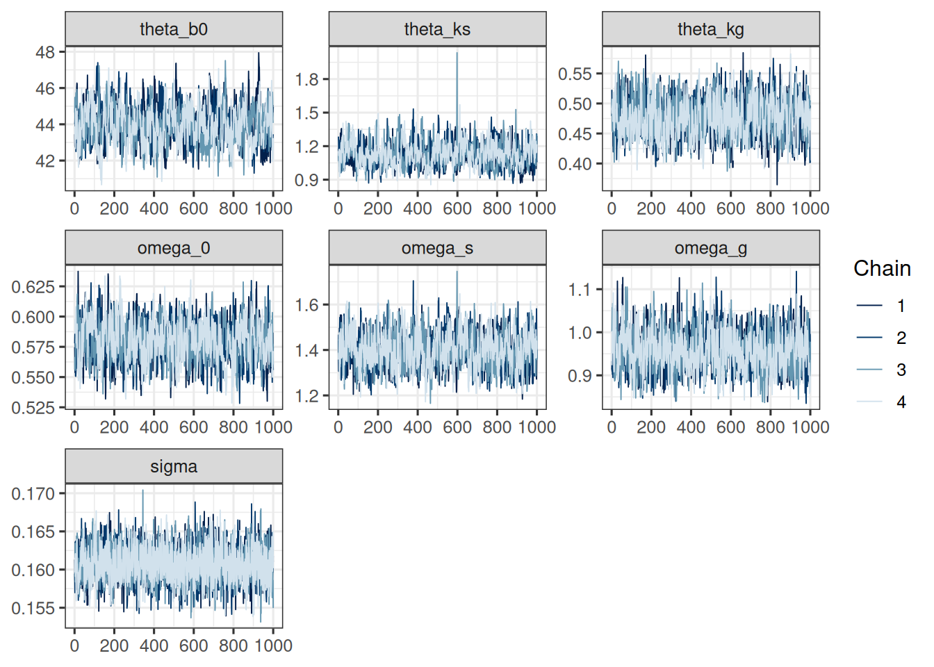
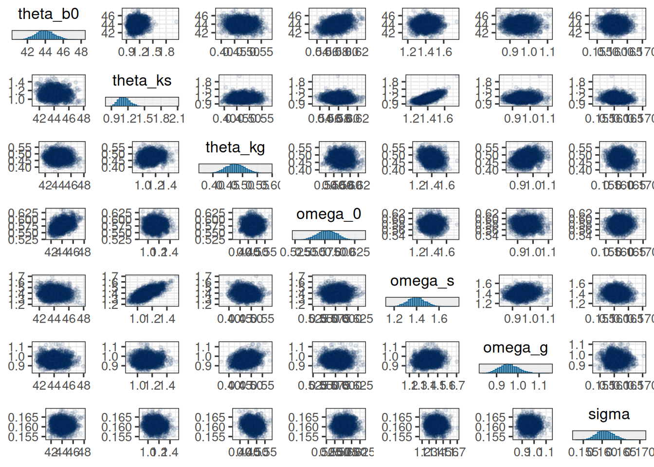
For a graphical check of the convergence, we can use the `mcmc_trace` and `mcmc_pairs` functions from the `bayesplot` package:
```{r}
#| label: plot_convergence
sf_pop_params <- c("theta_b0", "theta_ks", "theta_kg", "omega_0", "omega_s", "omega_g", "sigma")

mcmc_trace(post_df, pars = sf_pop_params)
mcmc_pairs(
  post_df,
  pars = sf_pop_params,
  off_diag_args = list(size = 1, alpha = 0.1)
)
```
Next, we can create a nice summary table of the parameter estimates, using `summarize_draws` from the `posterior` package in combination with functions from the `gt` package:
```{r}
#| label: summarize_parameters
post_sum <- post_df |>
  select(theta_b0, theta_ks, theta_kg, omega_0, omega_s, omega_g, cv_0, cv_s, cv_g, sigma) |>
  summarize_draws() |>
  gt() |>
  fmt_number(n_sigfig = 3)
post_sum
```
We can also look at parameters for individual patients. This is simplified by using the `spread_draws()` function:
```{r}
#| label: extract_individual_parameters
# Understand the names of the random effects:
head(get_variables(fit), 10)
post_ind <- fit |>
  spread_draws(
    b_lb0_Intercept,
    r_id__lb0[id, ],
    b_lks_Intercept,
    r_id__lks[id, ],
    b_lkg_Intercept,
    r_id__lkg[id, ]
  ) |>
  mutate(
    b0 = exp(b_lb0_Intercept + r_id__lb0),
    ks = exp(b_lks_Intercept + r_id__lks),
    kg = exp(b_lkg_Intercept + r_id__lkg)
  ) |>
  select(
    .chain, .iteration, .draw,
    id, b0, ks, kg
  )
```
Note that here we do *not* need to use the log-normal expectation formula, because we just calculate the individual random effects here, in contrast to the population level parameters above.
With this we can e.g. report the estimates for the first patient:
```{r}
#| label: first_patient_estimates
post_sum_id1 <- post_ind |>
  filter(id == "1") |>
  summarize_draws() |>
  gt() |>
  fmt_number(n_sigfig = 3)
post_sum_id1
```
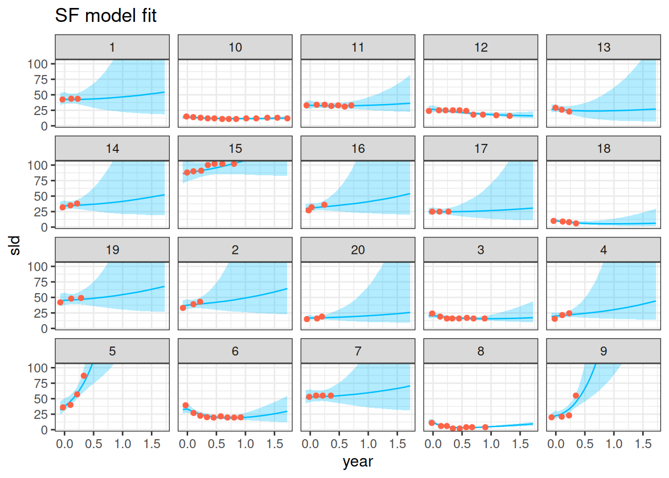
## Observation vs model fit
We can now compare the model fit to the observations. Let's do this for the first 20 patients again.
```{r}
#| label: obs_vs_fit_plots
pt_subset <- as.character(1:20)
df_subset <- df |>
  filter(id %in% pt_subset)

df_sim <- df_subset |>
  data_grid(
    id = pt_subset,
    year = seq_range(year, 101)
  ) |>
  add_linpred_draws(fit) |>
  median_qi() |>
  mutate(sld_pred = .linpred)

df_sim |>
  ggplot(aes(x = year, y = sld)) +
  facet_wrap(~ id) +
  geom_ribbon(
    aes(y = sld_pred, ymin = .lower, ymax = .upper),
    alpha = 0.3,
    fill = "deepskyblue"
  ) +
  geom_line(aes(y = sld_pred), color = "deepskyblue") +
  geom_point(data = df_subset, color = "tomato") +
  coord_cartesian(ylim = range(df_subset$sld)) +
  scale_fill_brewer(palette = "Greys") +
  labs(title = "SF model fit")
```
## Summary statistics
The time-to-growth formula is:
$$
\max \left(
\frac{
\log(k_s) - \log(k_g)
}{
k_s + k_g
},
0
\right)
$$
Similary, we can look at the tumor-ratio at time $t$:
$$
\frac{y^{*}(t)}{y^{*}(0)} = \exp(-k_s \cdot t) + \exp(k_g \cdot t) - 1
$$
So with the posterior samples from above, we can calculate these statistics, separate for each patient, with the tumor-ratio e.g. for 12 weeks (and being careful with the year time scale we used in this model):
```{r}
#| label: post_ind_stats
post_ind_stat <- post_ind |>
  mutate(
    ttg = pmax((log(ks) - log(kg)) / (ks + kg), 0),
    tr12 = exp(-ks * 12/52) + exp(kg * 12/52) - 1
  )
```
Then we can look at e.g. the first 3 patients parameter estimates:
```{r}
#| label: post_ind_stat_sum
post_ind_stat_sum <- post_ind_stat |>
  filter(id %in% c("1", "2", "3")) |>
  summarize_draws() |>
  gt() |>
  fmt_number(n_sigfig = 3)
post_ind_stat_sum
```
## Adding covariates
With `brms` it is straightforward to add covariates to the model. In this example, an obvious choice for a covariate is the treatment the patients received in the study:
```{r}
#| label: arms_distribution
df |>
  select(id, arm) |>
  distinct() |>
  pull(arm) |>
  table()
```
Here it makes sense to assume that only the shrinkage and growth parameters differ systematically between the two arms. For example, the baseline SLD should be the same in expectation, because of the randomization between the treatment arms.
Therefore we can add this binary `arm` covariate as follows as a fixed effect for the two population level mean parameters $\mu_{k_s}$ and $\mu_{k_g}$ on the log scale:
```{r}
#| label: formula_covariates
formula_by_arm <- bf(sld ~ ystar, nl = TRUE) +
  # Define the mean for the likelihood:
  nlf(
    ystar ~
      int_step(year > 0) *
        (b0 * (exp(-ks * year) + exp(kg * year) -  1)) +
      int_step(year <= 0) *
        (b0 * exp(kg * year))
  ) +
  # As above we also use these formulas here:
  nlf(sigma ~ log(tau) + log(ystar)) +
  lf(tau ~ 1) +
  # Define nonlinear parameter transformations:
  nlf(b0 ~ exp(lb0)) +
  nlf(ks ~ exp(lks)) +
  nlf(kg ~ exp(lkg)) +
  # Define random effect structure:
  lf(lb0 ~ 1 + (1 | id)) +
  lf(lks ~ 1 + arm + (1 | id)) +
  lf(lkg ~ 1 + arm + (1 | id))
```
It is instructive to see that the Stan code that is generated in the background is actually identical to the previous model, except for the prior specification. This is because `brms` uses a design matrix to model the fixed effects, and the `arm` variable is just added to this design matrix, which before only contained the intercept column with `1`s.
However, now the coefficient vector is no longer of length 1 but of length 2, with the first element corresponding to the intercept and the second element to the effect of the `arm` variable (for the level "2"). For the latter, we want to assume a standard normal prior on the log scale.
So we need to adjust the prior and initial values accordingly:
```{r}
#| label: priors_covariates
priors_by_arm <- c(
  prior(normal(log(65), 1), nlpar = "lb0"),
  # Note the changes here:
  prior(normal(log(0.52), 0.1), nlpar = "lks", coef = "Intercept"),
  prior(normal(0, 1), nlpar = "lks", coef = "arm2"),
  prior(normal(log(1.04), 1), nlpar = "lkg", coef = "Intercept"),
  prior(normal(0, 1), nlpar = "lkg", coef = "arm2"),
  # Same as before:
  prior(normal(0, 3), lb = 0, nlpar = "lb0", class = "sd"),
  prior(normal(0, 3), lb = 0, nlpar = "lks", class = "sd"),
  prior(normal(0, 3), lb = 0, nlpar = "lkg", class = "sd"),
  prior(normal(0, 3), lb = 0, nlpar = "tau")
)
inits_by_arm <- list(
  b_lb0 = array(3.61),
  # Note the changes here:
  b_lks = array(c(-1.25, 0)),
  b_lkg = array(c(-1.33, 0)),
  # Same as before:
  sd_1 = array(0.58),
  sd_2 = array(1.6),
  sd_3 = array(0.994),
  b_tau = array(0.161),
  z_1 = matrix(0, nrow = 1, ncol = n_patients),
  z_2 = matrix(0, nrow = 1, ncol = n_patients),
  z_3 = matrix(0, nrow = 1, ncol = n_patients)
)
```
Now we can fit the model as before:
```{r}
#| label: fit_brms_by_arm
save_file <- here("session-tgi/fit10.RData")
if (file.exists(save_file)) {
  load(save_file)
} else {
  fit_by_arm <- brm(
    formula = formula_by_arm,
    data = df,
    prior = priors_by_arm,
    family = gaussian(),
    init = rep(list(inits_by_arm), CHAINS),
    chains = CHAINS,
    iter = ITER + WARMUP,
    warmup = WARMUP,
    seed = BAYES.SEED,
    refresh = REFRESH
  )
  save(fit_by_arm, file = save_file)
}
summary(fit_by_arm)
```
Let's have a look at the parameter estimates then:
```{r}
#| label: extract_parameters_by_arm
post_df_by_arm <- as_draws_df(fit_by_arm)
head(names(post_df_by_arm), 10)
post_df_by_arm <- post_df_by_arm |>
  mutate(
    theta_b0 = exp(b_lb0_Intercept + sd_id__lb0_Intercept^2 / 2),
    theta_ks_arm1 = exp(b_lks_Intercept + sd_id__lks_Intercept^2 / 2),
    theta_ks_arm2 = exp(b_lks_Intercept + b_lks_arm2 + sd_id__lks_Intercept^2 / 2),
    theta_kg_arm1 = exp(b_lkg_Intercept + sd_id__lkg_Intercept^2 / 2),
    theta_kg_arm2 = exp(b_lkg_Intercept + b_lkg_arm2 + sd_id__lkg_Intercept^2 / 2),
    omega_0 = sd_id__lb0_Intercept,
    omega_s = sd_id__lks_Intercept,
    omega_g = sd_id__lkg_Intercept,
    cv_0 = sqrt(exp(sd_id__lb0_Intercept^2) - 1),
    cv_s = sqrt(exp(sd_id__lks_Intercept^2) - 1),
    cv_g = sqrt(exp(sd_id__lkg_Intercept^2) - 1),
    sigma = b_tau_Intercept
  )

post_sum_by_arm <- post_df_by_arm |>
  select(
    theta_b0, theta_ks_arm1, theta_ks_arm2, theta_kg_arm1, theta_kg_arm2,
    omega_0, omega_s, omega_g, cv_0, cv_s, cv_g, sigma
  ) |>
  summarize_draws() |>
  gt() |>
  fmt_number(n_sigfig = 3)
post_sum_by_arm
```
So we see that the shrinkage is stronger in arm 1 compared to arm 2, while the growth rates are similar. We could also calculate the posterior probability that the growth rate is different between the two arms, for example:
```{r}
#| label: posterior_prob_diff
post_df_by_arm |>
  mutate(diff_pos = theta_ks_arm1 - theta_ks_arm2 > 0) |>
  summarize(diff_prob = mean(diff_pos))
```
So we see that the posterior probability that the shrinkage rate is higher in arm 1 compared to arm 2 is quite high.
## Model comparison with LOO
The LOO criterion is a widely used method for comparing models. It is based on the idea of leave-one-out cross-validation, but is more efficient to compute.
With `brms`, it is easy to compute the LOO criterion:
```{r}
#| label: loo
loo(fit)
```
A helpful glossary explaining the LOO statistics can be found [here](https://mc-stan.org/cmdstanr/reference/loo-glossary.html).
Different criteria are available, for example the `elpd_loo` is the expected log pointwise predictive density, and the `looic = -2 * elpd_loo` is the LOO information criterion. For comparing models, the `looic` is often used, where smaller numbers are better. it is kind of an equivalent to the AIC, but based on the LOO criterion.
Let's e.g. compare the two models we fitted above, one for the whole dataset and one with the treatment arm as a covariate for the shrinkage and growth rates:
```{r}
#| label: loo_compare
fit <- add_criterion(fit, "loo")
fit_by_arm <- add_criterion(fit_by_arm, "loo")
loo_compare(fit, fit_by_arm)
```
So the model without treatment arm seems to be very slightly preferred here by the LOO criterion. Nevertheless, the model with treatment arm might answer exactly the question we need to answer, so it is important to consider the context of the analysis.
## Tips and tricks
- When the model breaks down completely, that is a sign that likely the model specification is wrong. For example, in above code I first did not understand how to model the `sigma` parameter correctly, which led to a model where each chain was completely stuck at its initial values.
- In that case and in general if you are not sure whether the `brms` model specification is correct, you can check the Stan code that is generated by `brms`:
```{r}
#| label: check_stan_code
# Good to check the stan code:
# (This also helps to find the names of the parameters
# for which to define the initial values below)
stancode(formula, prior = priors, data = df, family = gaussian())
```
Here e.g. it is important to see that the `sigma` parameter is modelled on the log scale.
- We can also extract the actual data that is passed to the Stan program:
```{r}
#| label: extract_data
# Extract the data that is passed to the Stan program
stan_data <- standata(formula, prior = priors, data = df, family = gaussian())

# Check that the time variable is correct
all(stan_data$C_eta_1 == df$year)
```
This can be useful to check if the data is passed correctly to the Stan program.
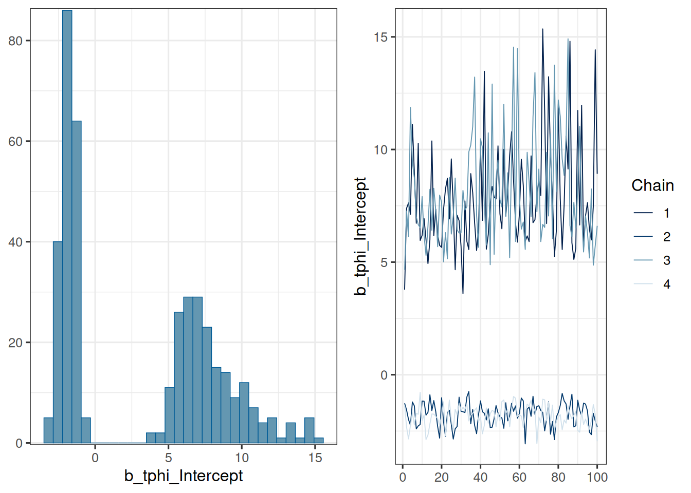
- It is important to take divergence warnings seriously. For the model parameters where `Rhat` is larger than 1.05 or so, you can just have a look at the traceplot. For example, in an earlier model fit the $\log(\mu_{\phi})$ population parameter had this traceplot:
```{r}
#| label: traceplot_example
fit_save <- fit
load(here("session-tgi/fit.RData"))
plot(fit, pars = "b_tphi")
fit <- fit_save
```
We see that two chains led to a $\log(\mu_{\phi})$ value below 0, while two chains hovered around much larger values between 5 and 15, which corresponds to $\mu_{\phi} = 1$. This shows that the model is rather overparametrized. By restricting the range of the prior for $\log(\mu_{\phi})$ to be below 0, we could avoid this problem.
- Providing manually realistic initial values for the model parameters can help to speed up the convergence of the Markov chains. This is especially important for the nonlinear parameters. You can get the names of the parameters from the Stan code above - note that you cannot use the names of the `brms` R code.
- Sometimes it is not easy to get the dimensions of the inital values right. Here it can be helpful to change the backend to `rstan`, which provides more detailed error messages. You can do this by setting `backend = "rstan"` in the `brm` call.
- When the Stan compiler gives you an error, that can be very informative: Just open the Stan code file that is mentioned in the error message and look at the line number that is mentioned. This can give you a good idea of what went wrong: Maybe a typo in the prior definition, or a missing semicolon, or a wrong dimension in the data block. With VScode e.g. this is very easy: Just hold `Ctrl` and click on the file name and number, and you will be taken to the right line in the Stan code.
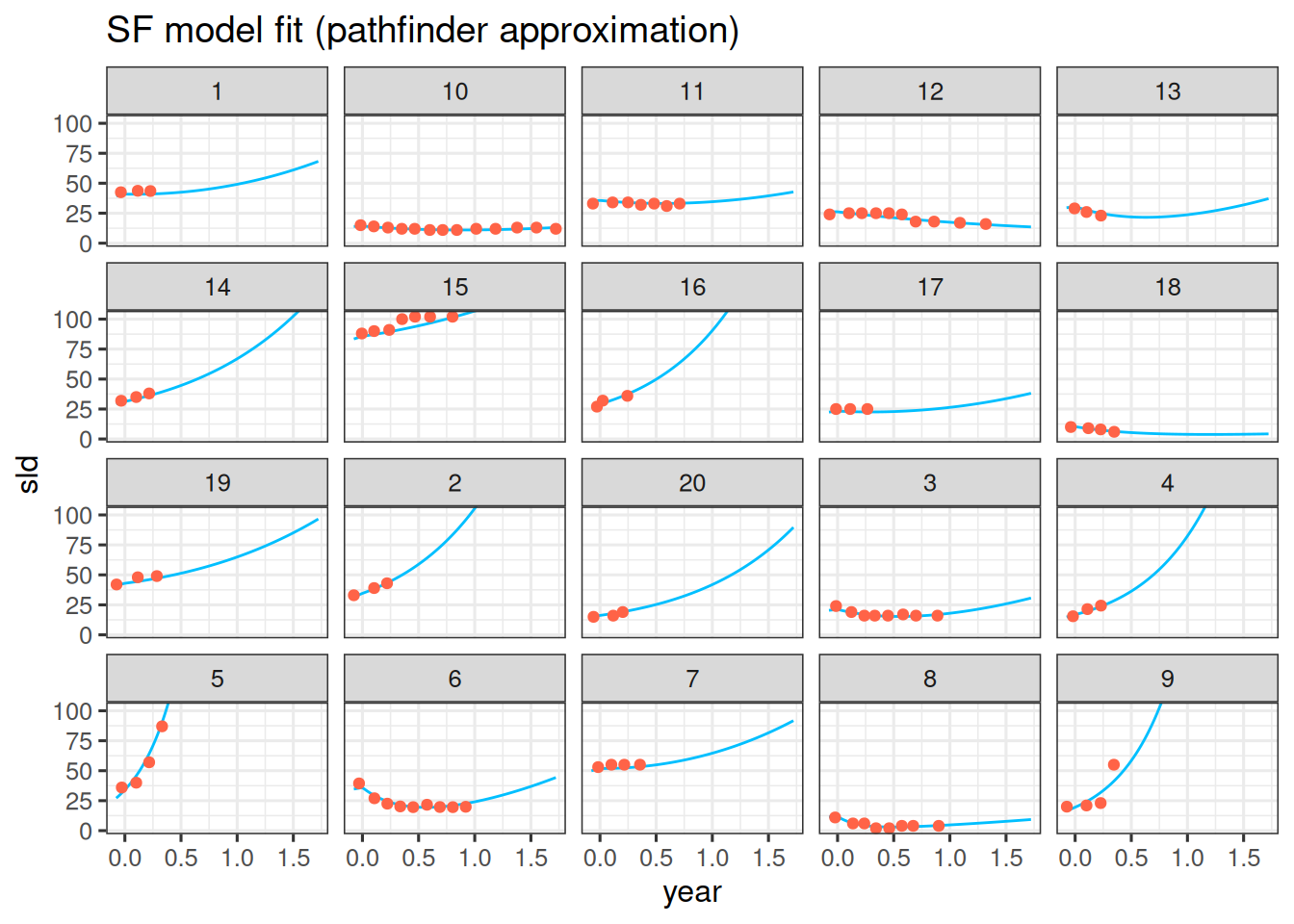
- In order to quickly get results for a model, e.g. for obtaining useful starting values or prior distributions, it can be worth trying the "Pathfinder" algorithm in `brms`. Pathfinder is a variational method for approximately sampling from differentiable log densities. You can use it by setting `algorithm = "pathfinder"` in the `brm` call. In this example it takes only a minute, compared to more than an hour for the full model fit. However, the results are still quite different, so it is likely only useful as a first approximation. Nevertheless, the individual model fits look quite encouraging, in the sense that they have found good parameter values - but they are still lacking any uncertainty, so could not be used for confidence or prediction intervals:
```{r}
#| label: fit_brms_pathfinder
fit_fast_file <- here("session-tgi/fit_fast.RData")
if (file.exists(fit_fast_file)) {
  load(fit_fast_file)
} else {
  fit_fast <- brm(
    formula = formula,
    data = df,
    prior = priors,
    family = gaussian(),
    init = rep(list(inits), CHAINS),
    chains = CHAINS,
    iter = ITER + WARMUP,
    warmup = WARMUP,
    seed = BAYES.SEED,
    refresh = REFRESH,
    algorithm = "pathfinder"
  )
  save(fit_fast, file = fit_fast_file)
}

summary(fit_fast)
df_sim <- df_subset |>
  data_grid(
    id = pt_subset,
    year = seq_range(year, 101)
  ) |>
  add_linpred_draws(fit_fast) |>
  median_qi() |>
  mutate(sld_pred = .linpred)

df_sim |>
  ggplot(aes(x = year, y = sld)) +
  facet_wrap(~ id) +
  geom_ribbon(
    aes(y = sld_pred, ymin = .lower, ymax = .upper),
    alpha = 0.3,
    fill = "deepskyblue"
  ) +
  geom_line(aes(y = sld_pred), color = "deepskyblue") +
  geom_point(data = df_subset, color = "tomato") +
  coord_cartesian(ylim = range(df_subset$sld)) +
  scale_fill_brewer(palette = "Greys") +
  labs(title = "SF model fit (pathfinder approximation)")
```