1. Calculate Bayesian Predictive Power

The purpose of this document is to show how we can calculate the probability of success given interim data of a clinical trial, based on the TGI-OS joint model results.

Setup and load data

Here we execute the R code from the setup and data preparation chapter, see the full code here.

Fit our joint TGI-OS model

Let’s fit again the same joint TGI-OS model as in the previous session. Now we just put all the code together in a single chunk, and it is a good repetition to see all the steps in one place:

subj_df <- os_data |>
    mutate(study = "OAK") |>
    select(study, id, arm)
subj_data <- DataSubject(
    data = subj_df,
    subject = "id",
    arm = "arm",
    study = "study"
)
long_df <- tumor_data |>
    select(id, year, sld)
long_data <- DataLongitudinal(
    data = long_df,
    formula = sld ~ year
)
surv_data <- DataSurvival(
    data = os_data,
    formula = Surv(os_time, os_event) ~ ecog + age + race + sex
)
joint_data <- DataJoint(
    subject = subj_data,
    longitudinal = long_data,
    survival = surv_data
)

joint_mod <- JointModel(
    longitudinal = LongitudinalSteinFojo(
        mu_bsld = prior_normal(log(65), 1),
        mu_ks = prior_normal(log(0.52), 1),
        mu_kg = prior_normal(log(1.04), 1),
        omega_bsld = prior_normal(0, 3) |> set_limits(0, Inf),
        omega_ks = prior_normal(0, 3) |> set_limits(0, Inf),
        omega_kg = prior_normal(0, 3) |> set_limits(0, Inf),
        sigma = prior_normal(0, 3) |> set_limits(0, Inf)
    ),
    survival = SurvivalWeibullPH(
        lambda = prior_gamma(0.7, 1),
        gamma = prior_gamma(1.5, 1),
        beta = prior_normal(0, 20)
    ),
    link = linkGrowth(
        prior = prior_normal(0, 20)
    )
)

options("jmpost.prior_shrinkage" = 0.99)
# initialValues(joint_mod, n_chains = CHAINS)

save_file <- here("session-pts/jm1.rds")
if (file.exists(save_file)) {
    joint_results <- readRDS(save_file)
} else {
    joint_results <- sampleStanModel(
        joint_mod,
        data = joint_data,
        iter_sampling = ITER,
        iter_warmup = WARMUP,
        chains = CHAINS,
        parallel_chains = CHAINS,
        thin = CHAINS,
        seed = BAYES.SEED,
        refresh = REFRESH
    )
    saveObject(joint_results, file = save_file)
}

Marginal Hazard Ratio Estimation

First, we will try to apply the methodology from Oudenhoven et al (2020) to estimate the marginal hazard ratio, using our joint model results. We use the new jmpost function called populationHR() for this:

save_file <- here("session-pts/jm1hr.rds")
if (file.exists(save_file)) {
    pop_hr <- readRDS(save_file)
} else {
    pop_hr <- populationHR(
        joint_results,
        hr_formula = ~arm
    )
    saveRDS(pop_hr, file = save_file)
}
pop_hr$summary

                          mean     median      X2.5.      X97.5.
bs(time, df = 10)1  -3.1898619 -3.1492166 -4.6595480 -1.94483471
bs(time, df = 10)2  -2.1685007 -2.1557204 -2.9129270 -1.44921371
bs(time, df = 10)3  -1.7541631 -1.7457712 -2.2606129 -1.27922919
bs(time, df = 10)4  -1.7402008 -1.7351076 -2.1929390 -1.32483535
bs(time, df = 10)5  -1.2832478 -1.2744974 -1.6118038 -0.99434352
bs(time, df = 10)6  -1.3567217 -1.3465337 -1.7256844 -1.02999961
bs(time, df = 10)7  -0.8752984 -0.8702259 -1.1870137 -0.60171732
bs(time, df = 10)8  -1.2314025 -1.2226766 -1.8595341 -0.71176107
bs(time, df = 10)9  -0.1212043 -0.1255963 -0.6237809  0.40773756
bs(time, df = 10)10 -0.5070327 -0.4897161 -1.1333247  0.02179326
armMPDL3280A        -0.2448721 -0.2361508 -0.5174069 -0.00558422

So here we have the marginal log hazard ratio estimates of the baseline spline components and the treatment arm. Therefore we can get the hazard ratio estimates by exponentiating the log hazard ratio estimates:

hr_est <- pop_hr$summary["armMPDL3280A", ] |>
    sapply(exp)

So we get a marginal hazard ratio estimate of around 0.783 and a 95% credible interval of 0.6 - 0.99.

Comparison with simple Cox PH results

We can do a little sanity check by comparing this with a very simple Cox model:

cox_mod <- survival::coxph(
    update(joint_results@data@survival@formula, ~ . + arm),
    data = joint_results@data@survival@data
)
summary(cox_mod)

Call:
survival::coxph(formula = update(joint_results@data@survival@formula, 
    ~. + arm), data = joint_results@data@survival@data)

  n= 203, number of events= 108 

                  coef exp(coef)  se(coef)      z Pr(>|z|)   
ecog1         0.617895  1.855019  0.209174  2.954  0.00314 **
age           0.002656  1.002659  0.009982  0.266  0.79018   
raceOTHER     0.602237  1.826200  0.400528  1.504  0.13268   
raceWHITE     0.082344  1.085829  0.229687  0.359  0.71997   
sexM          0.297556  1.346563  0.201567  1.476  0.13989   
armMPDL3280A -0.330645  0.718460  0.198119 -1.669  0.09513 . 
---
Signif. codes:  0 '***' 0.001 '**' 0.01 '*' 0.05 '.' 0.1 ' ' 1

             exp(coef) exp(-coef) lower .95 upper .95
ecog1           1.8550     0.5391    1.2311     2.795
age             1.0027     0.9973    0.9832     1.022
raceOTHER       1.8262     0.5476    0.8329     4.004
raceWHITE       1.0858     0.9210    0.6922     1.703
sexM            1.3466     0.7426    0.9071     1.999
armMPDL3280A    0.7185     1.3919    0.4873     1.059

Concordance= 0.621  (se = 0.027 )
Likelihood ratio test= 14.6  on 6 df,   p=0.02
Wald test            = 14.34  on 6 df,   p=0.03
Score (logrank) test = 14.63  on 6 df,   p=0.02

Here we get a different HR estimate of around 0.72, which is lower than the one we got from the joint model. We should expect different results because the joint model takes into account the TGI effect, while the Cox model does not.

And if we just put the treatment arm into the Cox model we get:

cox_mod_arm <- survival::coxph(
    update(joint_results@data@survival@formula, . ~ arm),
    data = joint_results@data@survival@data
)
cox_mod_arm

Call:
survival::coxph(formula = update(joint_results@data@survival@formula, 
    . ~ arm), data = joint_results@data@survival@data)

                coef exp(coef) se(coef)      z    p
armMPDL3280A -0.2414    0.7855   0.1928 -1.252 0.21

Likelihood ratio test=1.56  on 1 df, p=0.2109
n= 203, number of events= 108 

Here we get a HR of 0.785 that is close to the marginal HR estimate above (when we did not condition on the other covariates), which is reassuring. On the other hand, the 95% confidence interval is:

exp(confint(cox_mod_arm)["armMPDL3280A", ])

    2.5 %    97.5 % 
0.5383409 1.1461249 

so actually overlaps the null hypothesis of 1. So we see that the joint model helped us to obtain a more precise estimate of the marginal hazard ratio.

PTS based on frequentist HR properties

From now on we pretend that the data we have analyzed so far is the interim data of the Oak trial, and we want to calculate the predictive power of the trial based on this interim data.

Let’s first try to use the log HR (\(\delta\)) frequentist distribution to calculate the predictive power of the trial. We have:

\[ \hat{\delta}_{\text{fin}} \vert \hat{\delta}_{\text{int}} \sim \text{Normal}(\hat{\delta}_{\text{int}}, \sigma^2_{\text{int}}) \]

where the predictive variance is given by

\[ \sigma^2_{\text{int}} = \frac{1}{4\overline{p}r(1-r)} \frac{\overline{m}}{\overline{n} (\overline{n} + \overline{m})} \]

On the other hand, assuming that we have observed the final data, then the variance estimate for the estimator \(\hat{\delta}_{\text{fin}}\) is given by:

\[ \sigma^2_{\text{fin}} = \frac{1}{4\overline{p}r(1-r)} \frac{1}{\overline{n} + \overline{m}} \]

So the \((1-\alpha)\)-confidence interval for the final log HR is given by:

\[ \hat{\delta}_{\text{fin}} \pm z_{1 - \alpha/2} \sigma_{\text{fin}} \]

and the null hypothesis is rejected if the upper bound of this confidence interval is below 0, i.e. if:

\[ \hat{\delta}_{\text{fin}} + z_{1 - \alpha/2} \sigma_{\text{fin}} < 0. \]

Now let’s again take the perspective that we are at the interim analysis and we want to calculate the predictive probability of this event, then:

\[ \begin{align*} \mathbb{P}(\hat{\delta}_{\text{fin}} + z_{1 - \alpha/2} \sigma_{\text{fin}} < 0) &= \mathbb{P}(\hat{\delta}_{\text{fin}} < - z_{1 - \alpha/2} \sigma_{\text{fin}}) \\ &= \mathbb{P}\left( \frac{\hat{\delta}_{\text{fin}} - \hat{\delta}_{\text{int}}}{\sigma_{\text{int}}} < \frac{- z_{1 - \alpha/2} \sigma_{\text{fin}} - \hat{\delta}_{\text{int}}}{\sigma_{\text{int}}} \right) \\ &= \Phi\left( \frac{- z_{1 - \alpha/2} \sigma_{\text{fin}} - \hat{\delta}_{\text{int}}}{\sigma_{\text{int}}} \right) \end{align*} \]

because the left-hand side is a standard normal variable according to our formula above. Let’s first write a little function to calculate this:

pts_freq_hr <- function(delta_int, var_int, var_final, alpha = 0.05) {
    z_alpha <- qnorm(1 - alpha / 2)
    delta_final <- -z_alpha * sqrt(var_final)
    pnorm((delta_final - delta_int) / sqrt(var_int))
}

For \(\hat{\delta}_{\text{int}}\) we are going to plug in our MCMC samples for the marginal log HR \(\hat{\delta}_{\text{int}}\) to compute the PTS based on this:

log_hr_samples <- pop_hr[[2]]["armMPDL3280A", ]

But first we also need the quantities that go into the variance formula:

• \(\overline{p}\): average event rate
• \(r\): proportion of patients in the treatment arm
• \(\overline{n}\): average arm size in interim data
• \(\overline{m}\): average arm size in follow up

So let’s calculate these and the resulting variances:

avg_event_rate <- mean(os_data$os_event)
prop_pts_treatment <- mean(os_data$arm == "MPDL3280A")
avg_arm_size_interim <- mean(table(os_data$arm))
total_size_final <- 850
avg_arm_size_followup <- (total_size_final - 2 * avg_arm_size_interim) / 2
var_int <- 1 /
    (4 * avg_event_rate * prop_pts_treatment * (1 - prop_pts_treatment)) *
    avg_arm_size_followup /
    (avg_arm_size_interim * (avg_arm_size_interim + avg_arm_size_followup))
var_final <- 1 /
    (4 * avg_event_rate * prop_pts_treatment * (1 - prop_pts_treatment)) *
    1 /
    (avg_arm_size_interim + avg_arm_size_followup)

Now we can calculate the PTS based on the frequentist HR properties:

pts_freq_hr_result <- mean(pts_freq_hr(
    delta_int = log_hr_samples,
    var_int = var_int,
    var_final = var_final
))
pts_freq_hr_result

[1] 0.7318325

So we obtain a PTS of 73.2% here.

PTS based on frequentist log-rank test properties

Now we want to leverage the rpact function getConditionalPower() to calculate the predictive power of the trial based on the log-rank test statistic properties.

Looking at the function’s example, we first have to create a DataSet object with the interim data. Here it is important that we for cumLogRanks also the z scores from a Cox regression can be used, which means for our case that can insert here the z-scores defined as:

\[ z = \frac{\hat{\delta}_{\text{int}}}{\sigma_{\text{int}}} \]

values.

But let’s first try this with a simple fixed \(z\) value to see how it works:

library(rpact)

Installation qualification for rpact 4.2.1 has not yet been performed.

Please run testPackage() before using the package in GxP relevant environments.

z <- log(0.9) / sqrt(var_int) # Instead of log(0.9) we put later the marginal log HR MCMC sample
data <- getDataset(
    cumEvents = sum(os_data$os_event),
    cumLogRanks = z,
    cumAllocationRatios = prop_pts_treatment
)
data

Dataset of survival data

• Stages: 1
• Cumulative events: 108
• Cumulative allocation ratios: 0.527
• Cumulative log-ranks: -0.886

Calculated data

• Number of events: 108
• Allocation ratios: 0.527093596059113
• Log-ranks: -0.886

This is the data set from the first stage, i.e. our interim analysis.

Now we need to define the design of the group sequential trial:

events_final <- total_size_final * avg_event_rate
design <- getDesignGroupSequential(
    kMax = 2,
    informationRates = c(sum(os_data$os_event) / events_final, 1),
    alpha = 0.05
)
design

Design parameters and output of group sequential design

User defined parameters

• Information rates: 0.239, 1.000
• Significance level: 0.0500

Derived from user defined parameters

• Maximum number of stages: 2
• Stages: 1, 2
• Futility bounds (non-binding): -Inf

Default parameters

• Type of design: O’Brien & Fleming
• Type II error rate: 0.2000
• Binding futility: FALSE
• Test: one-sided
• Tolerance: 1e-08

Output

• Cumulative alpha spending: 0.000377, 0.050000
• Critical values: 3.369, 1.646
• Stage levels (one-sided): 0.000377, 0.049833

We see that the significance level is almost full for the final analysis, because by default the O’Brien & Fleming design is used, which only assigns a very small \(\alpha\) to the interim analysis. This is kind of what we need here.

Finally we put the design and data in a StageResults object, which is the input for the getConditionalPower() function:

stageResults <- getStageResults(
    design = design,
    dataInput = data,
    stage = 1,
    directionUpper = FALSE
)
condPower <- getConditionalPower(
    stageResults = stageResults,
    thetaH1 = 0.9, # Here we put later the marginal hazard ratio MCMC sample
    nPlanned = total_size_final,
    allocationRatioPlanned = 1
)
summary(condPower)

Technical developer summary of the Conditional power results survival object ("ConditionalPowerResultsSurvival"):

  [u] Planned sample size              : NA, 850 
  [d] Planned allocation ratio         : 1 
  [.] %simulated%                      : FALSE 
  [g] Conditional power                : NA, 0.5577 
  [u] Assumed effect under alternative : 0.9 

Legend:
  u: user defined
  >: derived value
  d: default value
  g: generated/calculated value
  .: not applicable or hidden

Conditional power results survival table:
     Planned sample size Conditional power
[1,]                  NA                NA
[2,]                 850         0.5576662

condPower$conditionalPower[2]

[1] 0.5576662

OK so now that we know how it works we wrap this in a little function again.

pts_freq_hr2 <- function(
    delta_int,
    var_int,
    var_final,
    events_int,
    alloc_int,
    events_final,
    alpha = 0.05) {
    data <- getDataset(
        cumEvents = events_int,
        cumLogRanks = delta_int / sqrt(var_int),
        cumAllocationRatios = alloc_int
    )
    design <- getDesignGroupSequential(
        kMax = 2,
        informationRates = c(events_int / events_final, 1),
        alpha = alpha
    )
    stageResults <- getStageResults(
        design = design,
        dataInput = data,
        stage = 1,
        directionUpper = FALSE
    )
    condPower <- getConditionalPower(
        stageResults = stageResults,
        thetaH1 = exp(delta_int),
        nPlanned = total_size_final,
        allocationRatioPlanned = 1
    )
    condPower$conditionalPower[2]
}

Let’s try it out with the same example first again:

pts_freq_hr2(
    delta_int = log(0.9),
    var_int = var_int,
    var_final = var_final,
    events_int = sum(os_data$os_event),
    alloc_int = prop_pts_treatment,
    events_final = total_size_final * avg_event_rate
)

[1] 0.5576662

OK so that gives the same result as before, which is good. Now we can plug in the MCMC samples for the marginal log HR:

save_file <- here("session-pts/jm1hr2.rds")
if (file.exists(save_file)) {
    pts_freq_hr2_samples <- readRDS(save_file)
} else {
    pts_freq_hr2_samples <- sapply(
        log_hr_samples,
        pts_freq_hr2,
        var_int = var_int,
        var_final = var_final,
        events_int = sum(os_data$os_event),
        alloc_int = prop_pts_treatment,
        events_final = total_size_final * avg_event_rate
    )
    saveRDS(pts_freq_hr2_samples, file = save_file)
}
pts_freq_hr2_result <- mean(pts_freq_hr2_samples)
pts_freq_hr2_result

[1] 0.8415316

So here we get a PTS of 84.2%, which is higher than the one we got before.

Individual Samples based Predictive Power

This is a good motivation to try out the conditional sampling approach to calculate the predictive power, which is based on the individual samples of the joint model. It does not involved any frequentist assumptions to calculate the PTS.

We will perform the following steps in this algorithm:

1. We add as many new patients to the survival data set as we expect to still enter the trial.
   • These patients have survival time 0 and are censored at that time, which means they are completely new patients.
2. We refit the joint model with this augmented data set. This simplifies the subsequent sampling process.
3. For each patient who is still being followed up for OS at IA (=does not have an event yet and did not drop out)
   • Obtain individual survival distribution MCMC samples over a long enough time grid
   • Condition on last observed censored OS time, sample once per MCMC sample from the conditional survival distribution
4. Define “End of Study” time, e.g. based on number of events observed, calendar time, etc.
5. Apply summary statistic of interest to the complete “End of Study” OS data set samples and aggregate appropriately
   • For example, we can use the log-rank test statistic as summary statistic
6. Calculate the proportion of samples that are above the critical value for the summary statistic, e.g. log-rank test statistic

Note that for the first step, we need to add some random information to the data set, because unfortunately the real data does not differentiate between patients who are still being followed up and those who have dropped out.

Add new patients and generate random lost-to-follow-up flag

Basically for those patients with a censored survival time, we randomly assign a lost-to-follow-up flag with a probability of 10%, so that we can simulate some patients who are still being followed up and some who are not. We sample the covariates from the distribution of the already observed patients.

set.seed(689)
lost_to_follow_up_flag <- sample(
    c(TRUE, FALSE),
    size = nrow(os_data),
    replace = TRUE,
    prob = c(0.1, 0.9)
)
os_data <- os_data |>
    mutate(lost_to_follow_up = !os_event & lost_to_follow_up_flag)
n_lost_to_follow_up <- sum(os_data$lost_to_follow_up)
n_lost_to_follow_up

[1] 10

set.seed(359)
n_new_patients <- 2 * avg_arm_size_followup
os_data_new <- data.frame(
    id = seq(from = max(as.integer(as.character(os_data$id))) + 1, length.out = n_new_patients),
    arm = rep(c("Docetaxel", "MPDL3280A"), c(floor(avg_arm_size_followup), ceiling(avg_arm_size_followup))),
    os_time = 0,
    os_event = FALSE,
    lost_to_follow_up = FALSE,
    ecog = sample(os_data$ecog, n_new_patients, replace = TRUE),
    age = sample(os_data$age, n_new_patients, replace = TRUE),
    race = sample(os_data$race, n_new_patients, replace = TRUE),
    sex = sample(os_data$sex, n_new_patients, replace = TRUE)
)
os_data_augmented <- os_data[, names(os_data_new)] |>
    mutate(id = as.character(id)) |>
    rbind(os_data_new) |>
    mutate(id = factor(id))

n_censored <- sum(!os_data_augmented$os_event & !os_data_augmented$lost_to_follow_up)
n_censored

[1] 732

So now we have 10 patients who have been lost to follow-up and 732 patients who are still being followed up for OS (or who will still be entering the trial). These 732 patients will be the ones we will perform the individual sampling for.

Refit the joint model with augmented data

First we need to refit the joint model to this augmented data set. That is the easiest way to also get survival curve samples for the patients who are yet to be enrolled in the trial.

We notice that here we also need to add at least some random baseline samples to the longitudinal data set, otherwise it does not work.

subj_aug_df <- os_data_augmented |>
    mutate(study = "OAK") |>
    select(study, id, arm)
subj_aug_data <- DataSubject(
    data = subj_aug_df,
    subject = "id",
    arm = "arm",
    study = "study"
)
long_df <- tumor_data |>
    select(id, year, sld)
new_long_df <- os_data_new |>
    select(id, os_time) |>
    rename(year = os_time) |>
    mutate(sld = sample(tumor_data$sld, n_new_patients, replace = TRUE))
long_aug_df <- long_df |>
    mutate(id = as.character(id)) |>
    rbind(new_long_df) |>
    mutate(id = factor(id))
stopifnot(identical(levels(long_aug_df$id), levels(subj_aug_df$id)))

long_aug_data <- DataLongitudinal(
    data = long_aug_df,
    formula = sld ~ year
)
surv_aug_data <- DataSurvival(
    data = os_data_augmented,
    formula = Surv(os_time, os_event) ~ ecog + age + race + sex
)
joint_aug_data <- DataJoint(
    subject = subj_aug_data,
    longitudinal = long_aug_data,
    survival = surv_aug_data
)

save_file <- here("session-pts/jm2.rds")
if (file.exists(save_file)) {
    joint_aug_results <- readRDS(save_file)
} else {
    joint_aug_results <- sampleStanModel(
        joint_mod,
        data = joint_aug_data,
        iter_sampling = ITER,
        iter_warmup = WARMUP,
        chains = CHAINS,
        parallel_chains = CHAINS,
        thin = CHAINS,
        seed = BAYES.SEED,
        refresh = REFRESH
    )
    saveObject(joint_aug_results, file = save_file)
}

Individual Sampling of OS events

Now we can perform the individual sampling of the OS events for the patients who are still being followed up. Let’s start with a single patient:

patient_id <- os_data_augmented |>
    filter(!os_event & !lost_to_follow_up) |>
    pull(id) |>
    unique() |>
    head(1)

So for this patient 588, we can extract the individual survival distribution MCMC samples from the joint model results along a time grid that extrapolates long enough into the future, say 10 years after the last observed OS time:

length_time_grid <- 100
time_grid_end <- round(max(os_data_augmented$os_time) + 10, 1)
time_grid <- seq(0, time_grid_end, length = length_time_grid)

save_file <- here("session-pts/jm2_surv_samples.rds")
if (file.exists(save_file)) {
    os_surv_samples <- readRDS(save_file)
} else {
    os_surv_samples <- SurvivalQuantities(
        object = joint_aug_results,
        grid = GridFixed(times = time_grid),
        type = "surv"
    )
    saveRDS(os_surv_samples, file = save_file)
}

os_surv_samples_df <- as.data.frame(os_surv_samples)
os_surv_samples_patient <- os_surv_samples_df |>
    filter(group == patient_id) |>
    select(-group) |>
    mutate(sample_id = rep(1:ITER, length_time_grid))
head(os_surv_samples_patient)

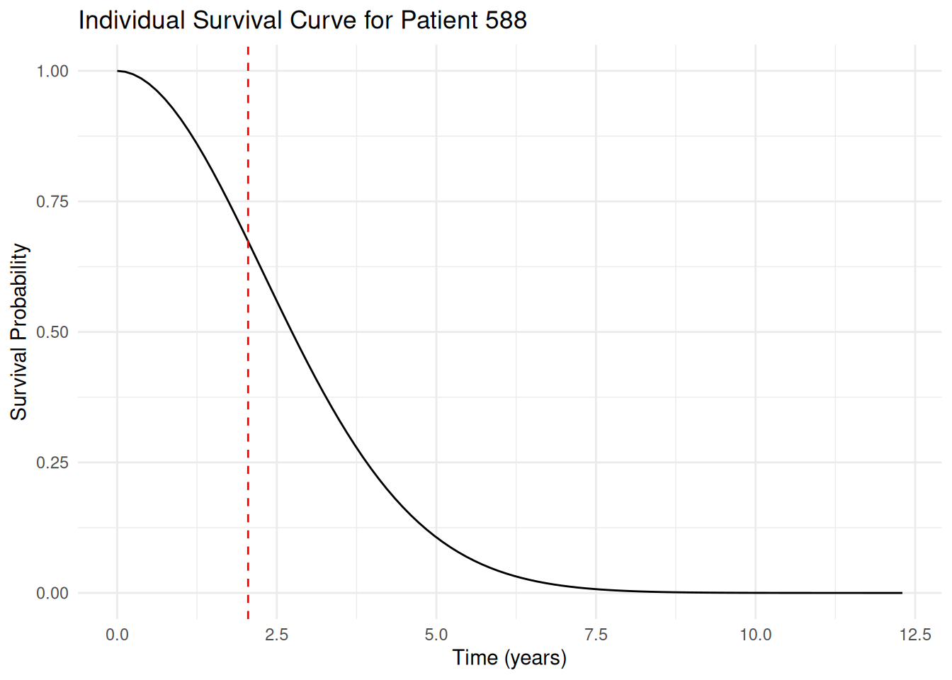
Now let’s zoom in on the first sampled survival curve of this patient, where we show also the last observed OS time as a vertical dashed line:

first_surv_sample <- os_surv_samples_patient |>
    filter(sample_id == 1)
patient_last_os_time <- os_data_augmented$os_time[os_data_augmented$id == patient_id]
first_surv_sample_plot <- ggplot(first_surv_sample, aes(x = time, y = values)) +
    geom_line() +
    labs(
        title = paste("Individual Survival Curve for Patient", patient_id),
        x = "Time (years)",
        y = "Survival Probability"
    ) +
    geom_vline(
        xintercept = patient_last_os_time,
        linetype = "dashed",
        color = "red"
    ) +
    theme_minimal()
first_surv_sample_plot

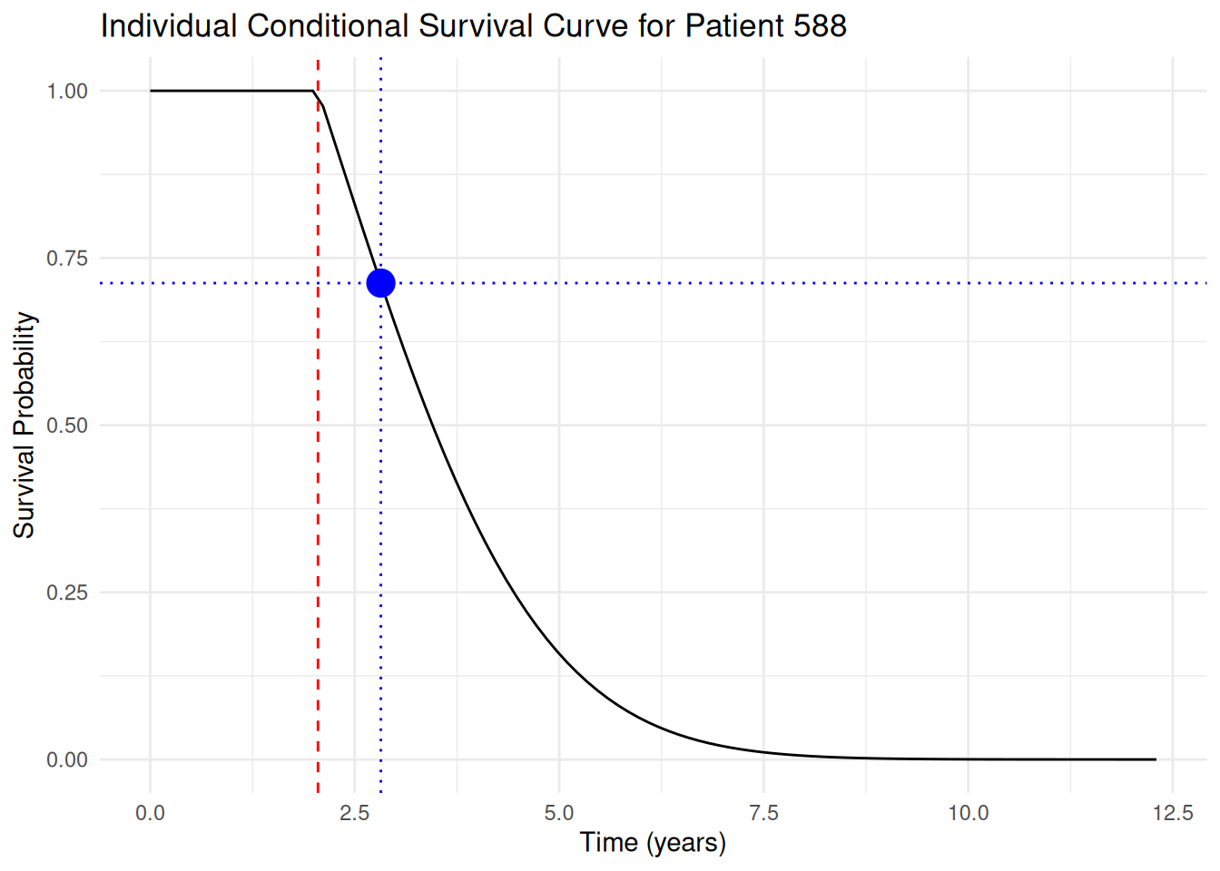
As described in the slides, we can now sample a survival time for this patient from the conditional survival distribution, given the last observed OS time, by:

1. Drawing a standard uniform random number \(p \sim U(0, 1)\)
2. Finding the time \(t\) such that \((1-p)S(c) - S(t) = 0\) where $c = 2.1 is the last observed OS time

set.seed(123)
p <- runif(1)

# Linear approximation function for the survival function:
surv_approx <- approxfun(
    x = first_surv_sample$time,
    y = first_surv_sample$values,
    rule = 2 # extrapolation outside interval via closest data extreme
)

# Survival function value at the time of censoring:
surv_at_censoring <- surv_approx(patient_last_os_time)

# Find the time t such that (1-p) * S(c) - S(t) = 0:
t <- uniroot(
    function(t) (1 - p) * surv_at_censoring - surv_approx(t),
    interval = c(0, time_grid_end)
)$root
t

[1] 2.819322

We can plot the conditional survival function together with this sampled survival time:

first_surv_sample <- first_surv_sample |>
    mutate(
        cond_values = ifelse(
            time <= patient_last_os_time,
            1,
            values / surv_at_censoring
        )
    )

first_cond_surv_sample_plot <- ggplot(
    first_surv_sample,
    aes(x = time, y = cond_values)
) +
    geom_line() +
    labs(
        title = paste(
            "Individual Conditional Survival Curve for Patient",
            patient_id
        ),
        x = "Time (years)",
        y = "Survival Probability"
    ) +
    geom_vline(
        xintercept = patient_last_os_time,
        linetype = "dashed",
        color = "red"
    ) +
    theme_minimal() +
    geom_vline(
        xintercept = t,
        linetype = "dotted",
        color = "blue"
    ) +
    geom_hline(
        yintercept = 1 - p,
        linetype = "dotted",
        color = "blue"
    ) +
    geom_point(
        data = data.frame(t = t, p = p),
        aes(x = t, y = 1 - p),
        color = "blue",
        size = 5
    )
first_cond_surv_sample_plot

The challenge is now to do this efficiently for all patients who are still being followed up for OS, and for all of their MCMC samples.

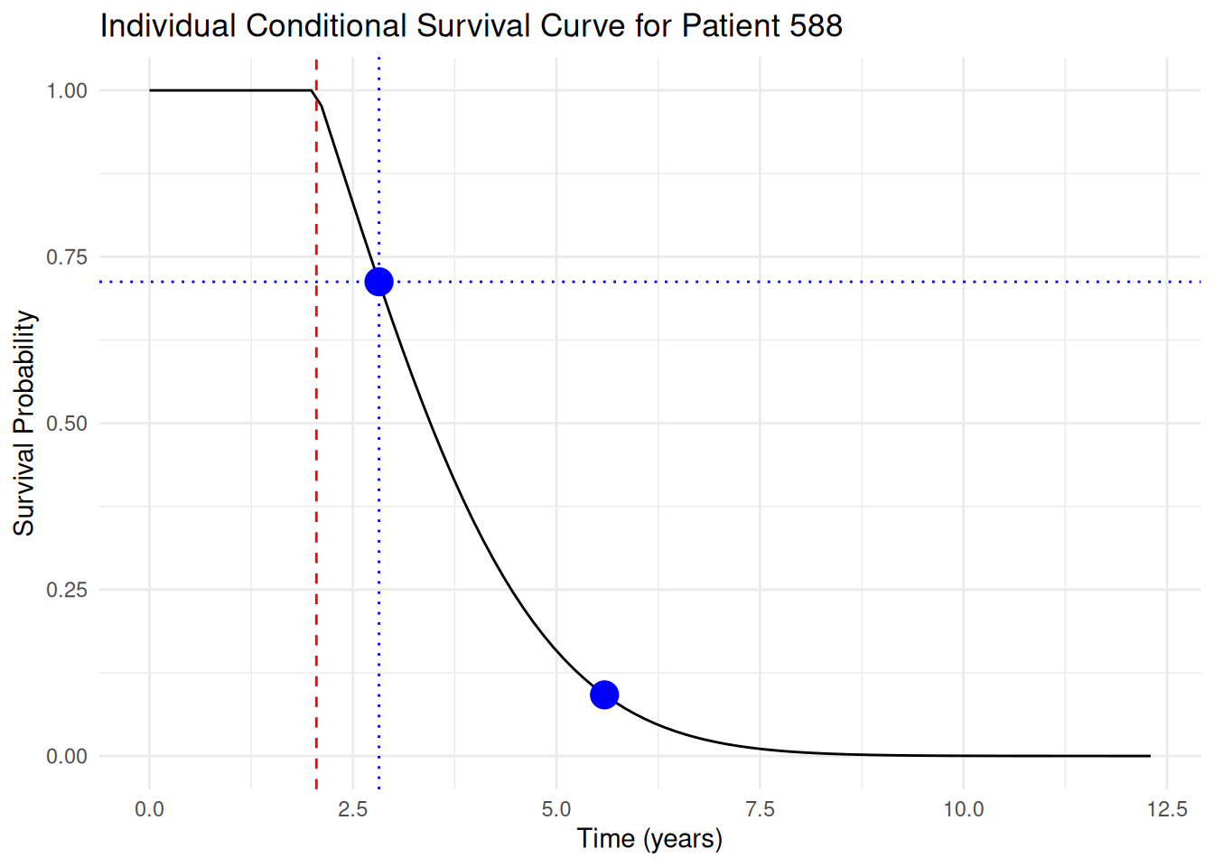
Simplified Rcpp implementation for single patient/sample

For now, let’s create a simpler Rcpp function that handles a single patient’s single MCMC sample:

library(Rcpp)

# Use Rcpp function for single patient, single sample.
sourceCpp(here("session-pts/conditional_sampling.cpp"))

# Test the function with a simple example.
set.seed(3453)

t_cpp_simple <- sample_single_conditional_survival_time(
    time_grid = first_surv_sample$time,
    surv_values = first_surv_sample$values,
    censoring_time = patient_last_os_time
)

first_cond_surv_sample_plot +
    geom_point(
        data = data.frame(
            t = t_cpp_simple$t_result,
            p = t_cpp_simple$uniform_sample
        ),
        aes(x = t, y = 1 - p),
        color = "blue",
        size = 5
    )

Rcpp implementation for all patients and samples

Let’s use the second Rcpp function that handles all patients and all MCMC samples at once. We just need to prepare the data in the right format:

• The first argument is the time grid, which we already have.
• The second argument is a matrix of survival values, where each row is a sample/patient combination and each column is a time point.
• The third argument is a vector of censoring times, where each element corresponds to a sample/patient combination.

# First subset to the patients where we need to sample from the conditional survival distribution.
pt_to_sample <- os_data_augmented |>
    filter(!os_event & !lost_to_follow_up)
pt_to_sample_ids <- pt_to_sample$id

qs <- os_surv_samples@quantities
include_qs <- qs@groups %in% pt_to_sample_ids

qs_samples <- qs@quantities[, include_qs]
qs_times <- qs@times[include_qs]
qs_groups <- qs@groups[include_qs]

surv_values_samples <- matrix(
    qs_samples,
    nrow = ITER * length(pt_to_sample_ids),
    ncol = length_time_grid
)
dim(surv_values_samples)

[1] 732000    100

surv_values_pt_ids <- rep(
    head(qs_groups, length(pt_to_sample_ids)),
    each = ITER
)

censoring_times <- pt_to_sample$os_time[match(
    surv_values_pt_ids,
    pt_to_sample_ids
)]
length(censoring_times)

[1] 732000

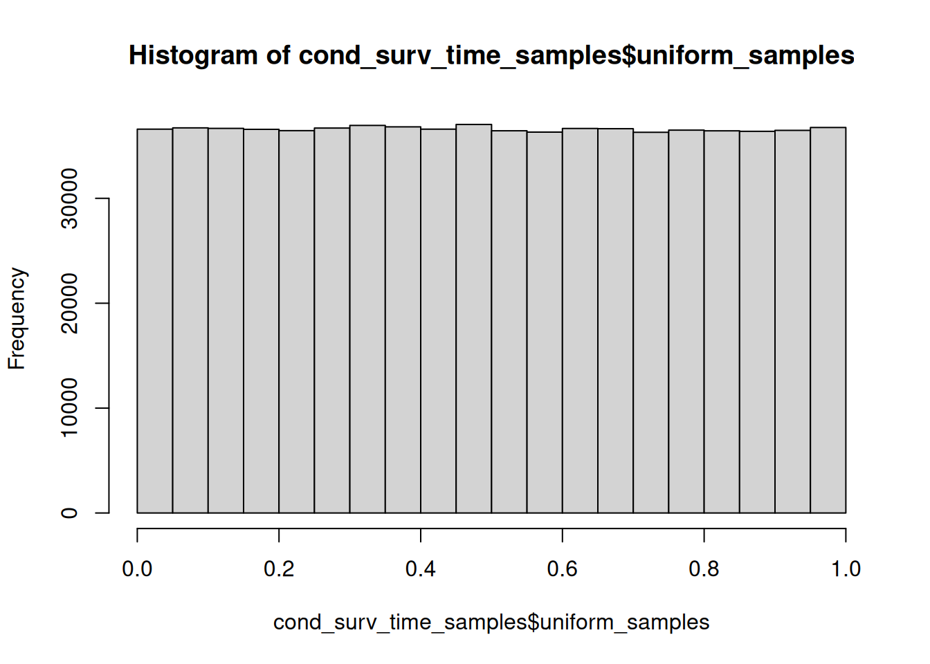
cond_surv_time_samples <- sample_conditional_survival_times(
    time_grid = time_grid,
    surv_values = surv_values_samples,
    censoring_times = censoring_times
)
mean(cond_surv_time_samples$beyond_max_time)

[1] 0.003687158

summary(cond_surv_time_samples$t_results)

     Min.   1st Qu.    Median      Mean   3rd Qu.      Max. 
1.170e-05 9.700e-01 1.793e+00 2.221e+00 2.889e+00 1.230e+01 

hist(cond_surv_time_samples$uniform_samples)

os_cond_samples <- matrix(
    cond_surv_time_samples$t_results,
    nrow = ITER,
    ncol = length(pt_to_sample_ids),
    dimnames = list(seq_len(ITER), head(qs_groups, length(pt_to_sample_ids)))
)

So this function is very fast, and in this case we have less than 1% of the samples where we did not have a long enough time grid, which seems sufficient for our purposes.

Generating OS data set samples

Now that we have the OS events for the patients who are still being followed up, we can generate the complete OS data set samples for each MCMC sample.

# Where do we need to replace the OS times?
os_rows_to_replace <- match(
    pt_to_sample_ids,
    os_data_augmented$id
)

# From which column do we take the sampled OS times?
os_cond_samples_cols <- match(
    pt_to_sample_ids,
    colnames(os_cond_samples)
)

os_data_samples <- lapply(1:ITER, function(i) {
    # Create a copy of the original OS data
    os_data_sample <- os_data_augmented[, c("id", "arm", "os_time", "os_event", "race", "sex", "ecog", "age")]

    # Add the sampled OS times for the patients who are still being followed up.
    os_data_sample$os_time[os_rows_to_replace] <- os_cond_samples[
        i,
        os_cond_samples_cols
    ]

    # Set the OS event to TRUE for those patients, because we assume they have an event now.
    os_data_sample$os_event[os_rows_to_replace] <- TRUE

    os_data_sample
})

Calculate log rank statistic for each sampled OS data set

Now it is easy to calculate the log-rank test statistic for each sampled OS data set. Here we don’t adjust for any covariates.

log_rank_stats_fun <- function(df) {
    surv_diff <- survival::survdiff(
        Surv(os_time, os_event) ~ arm,
        data = df
    )
    surv_diff$chisq
}

log_rank_stats <- sapply(os_data_samples, log_rank_stats_fun)
hist(log_rank_stats)

log_rank_at_ia <- log_rank_stats_fun(os_data_augmented)
log_rank_at_ia

[1] 1.584927

abline(v = log_rank_at_ia, col = "red", lwd = 2)
critical_value <- qchisq(0.95, df = 1)
abline(v = critical_value, col = "blue", lwd = 2)

And using the critical value of the log-rank test statistic for a significance level of 0.05, we can calculate the PTS:

pts_log_rank <- mean(log_rank_stats > critical_value)
pts_log_rank

[1] 0.693

So we see that this PTS with 69.3% is a bit lower than the previous PTS estimates.

Hazard Ratio based PTS

We can also calculate the PTS in an analogous way using the hazard ratio estimates:

hr_pval_fun <- function(df) {
    cox_mod <- survival::coxph(
        Surv(os_time, os_event) ~ arm + ecog + age + race + sex,
        data = df
    )
    summary(cox_mod)$coefficients[1, 5]
}

hr_pvals <- sapply(os_data_samples, hr_pval_fun)

pts_hr <- mean(hr_pvals < 0.05)
pts_hr

[1] 0.828

In this PTS estimate we can adjust for the covariates. We see that the result of 82.8% is in line with the frequentist based PTS estimate for the HR which we calculated earlier.

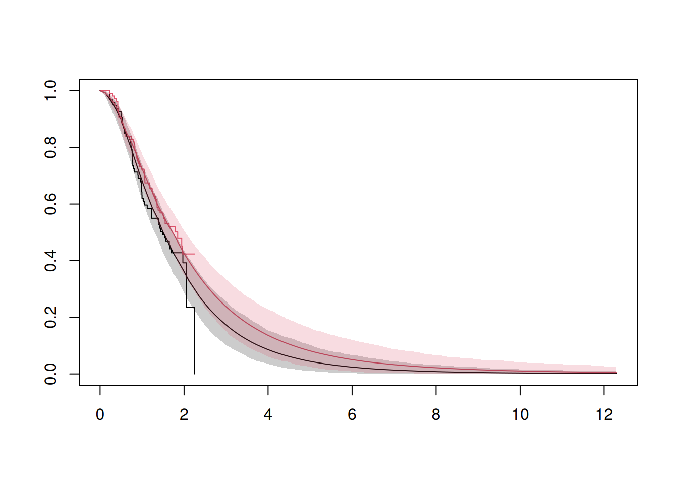
Plot Kaplan-Meier curves predictions

Similarly we can extract the Kaplan-Meier curves for each sampled OS data set and plot them:

km_curves <- lapply(os_data_samples, function(df) {
    survfit_obj <- survival::survfit(Surv(os_time, os_event) ~ arm, data = df)
    times <- survfit_obj$time
    surv_probs <- survfit_obj$surv
    strata <- survfit_obj$strata
    n_control <- strata[1]
    n_treatment <- strata[2]

    control_fun <- stepfun(
        times[1:n_control],
        c(1, surv_probs[1:n_control]),
        right = TRUE
    )
    treatment_fun <- stepfun(
        times[(n_control + 1):length(times)],
        c(1, surv_probs[(n_control + 1):length(surv_probs)]),
        right = TRUE
    )
    control_vals <- control_fun(time_grid)
    treatment_vals <- treatment_fun(time_grid)

    list(control = control_vals, treatment = treatment_vals)
})

km_control_samples <- sapply(km_curves, function(x) x$control)
km_treatment_samples <- sapply(km_curves, function(x) x$treatment)

survfit_ia <- survival::survfit(Surv(os_time, os_event) ~ arm, data = os_data_augmented)

plot(survfit_ia, col = c(1, 2), xlim = c(0, max(time_grid)))

# Add the mean KM curves for each arm.
lines(time_grid, rowMeans(km_control_samples), col = 1)
lines(time_grid, rowMeans(km_treatment_samples), col = 2)

# Add pointwise confidence intervals as shaded areas.
km_control_ci <- apply(km_control_samples, 1, quantile, probs = c(0.025, 0.975))
km_treatment_ci <- apply(
    km_treatment_samples,
    1,
    quantile,
    probs = c(0.025, 0.975)
)

polygon(
    c(time_grid, rev(time_grid)),
    c(km_control_ci[1, ], rev(km_control_ci[2, ])),
    col = adjustcolor(1, alpha.f = 0.2),
    border = NA
)
polygon(
    c(time_grid, rev(time_grid)),
    c(km_treatment_ci[1, ], rev(km_treatment_ci[2, ])),
    col = adjustcolor(2, alpha.f = 0.2),
    border = NA
)

We can see that we assume a very long follow up of the data here. Obviously we could cut the data sets at a certain number of events or a specific time point easily.