2. OS model minimal workflow with brms

Let’s try to fit the same model now with brms. We will use the same data as in the previous notebook.

Setup and load data

Here we directly start from the overall survival data with the log kg estimates, as we have obtained them in the previous notebook:

os_data_with_log_kg <- readRDS(here("session-os/os_data_with_log_kg.rds"))
head(os_data_with_log_kg)

# A tibble: 6 × 9
  id    arm       ecog    age race  sex   os_time os_event log_kg_est
  <fct> <fct>     <fct> <dbl> <fct> <fct>   <dbl> <lgl>         <dbl>
1 588   Docetaxel 0        61 WHITE F       2.05  FALSE       -0.571 
2 330   MPDL3280A 1        56 WHITE F       1.68  FALSE       -1.89  
3 791   Docetaxel 0        72 WHITE F       0.901 TRUE        -0.518 
4 635   Docetaxel 0        42 OTHER F       1.66  TRUE        -0.642 
5 365   MPDL3280A 0        64 WHITE F       1.43  TRUE        -0.427 
6 773   Docetaxel 0        65 WHITE M       1.63  FALSE        0.0340

Model fitting with brms

Let’s first fit the model with brms. We will use the same (first) model as in the previous notebook, but we will use the brms package to fit it.

An important ingredient for the model formula is the censoring information, passed via the cens() syntax: This should point to a variable containing the value 0 for observed events, i.e. no censoring, and the value 1 for right censored times (see ?brmsformula for more details). Therefore we first add such a variable to the data set:

os_data_with_log_kg <- os_data_with_log_kg |>
    mutate(
        os_cens = ifelse(os_event, 0, 1)
    )

We define our own design matrix with a column of ones:

os_data_with_log_kg_design <- model.matrix(
    ~ os_time + os_cens + ecog + age + race + sex + log_kg_est,
    data = os_data_with_log_kg
) |>
    as.data.frame() |>
    rename(ones = "(Intercept)")
head(os_data_with_log_kg_design)

  ones   os_time os_cens ecog1 age raceOTHER raceWHITE sexM  log_kg_est
1    1 2.0506502       1     0  61         0         1    0 -0.57141474
2    1 1.6755647       1     1  56         0         1    0 -1.88737445
3    1 0.9007529       0     0  72         0         1    0 -0.51807234
4    1 1.6591376       0     0  42         1         0    0 -0.64165688
5    1 1.4291581       0     0  64         0         1    0 -0.42656542
6    1 1.6290212       1     0  65         0         1    1  0.03404769

Now we can define the model formula:

formula <- bf(
    os_time | cens(os_cens) ~
        0 +
        ones +
        ecog1 +
        age +
        raceOTHER +
        raceWHITE +
        sexM +
        log_kg_est
)

So here we suppress the automatic intercept provided by brms by using the 0 + syntax, and instead we our “own” vector of ones. This is because we want to avoid the default centering of covariates which is performed by brms when using an automatic intercept. Otherwise it would be difficult to exactly match the prior distributions we used in the jmpost model further below.

In order to find out about the parametrization of the Weibull model with brms and Stan here, let’s check the Stan code generated by brms for it:

stancode(formula, data = os_data_with_log_kg_design, family = weibull())

// generated with brms 2.23.0
functions {
}
data {
  int<lower=1> N;  // total number of observations
  vector[N] Y;  // response variable
  // censoring indicator: 0 = event, 1 = right, -1 = left, 2 = interval censored
  array[N] int<lower=-1,upper=2> cens;
  int<lower=1> K;  // number of population-level effects
  matrix[N, K] X;  // population-level design matrix
  int prior_only;  // should the likelihood be ignored?
}
transformed data {
  // indices of censored data
  int Nevent = 0;
  int Nrcens = 0;
  int Nlcens = 0;
  array[N] int Jevent;
  array[N] int Jrcens;
  array[N] int Jlcens;
  // collect indices of censored data
  for (n in 1:N) {
    if (cens[n] == 0) {
      Nevent += 1;
      Jevent[Nevent] = n;
    } else if (cens[n] == 1) {
      Nrcens += 1;
      Jrcens[Nrcens] = n;
    } else if (cens[n] == -1) {
      Nlcens += 1;
      Jlcens[Nlcens] = n;
    }
  }
}
parameters {
  vector[K] b;  // regression coefficients
  real<lower=0> shape;  // shape parameter
}
transformed parameters {
  // prior contributions to the log posterior
  real lprior = 0;
  lprior += gamma_lpdf(shape | 0.01, 0.01);
}
model {
  // likelihood including constants
  if (!prior_only) {
    // initialize linear predictor term
    vector[N] mu = rep_vector(0.0, N);
    mu += X * b;
    mu = exp(mu);
    // vectorized log-likelihood contributions of censored data
    target += weibull_lpdf(Y[Jevent[1:Nevent]] | shape, mu[Jevent[1:Nevent]] ./ tgamma(1 + 1 ./ shape));
    target += weibull_lccdf(Y[Jrcens[1:Nrcens]] | shape, mu[Jrcens[1:Nrcens]] ./ tgamma(1 + 1 ./ shape));
    target += weibull_lcdf(Y[Jlcens[1:Nlcens]] | shape, mu[Jlcens[1:Nlcens]] ./ tgamma(1 + 1 ./ shape));
  }
  // priors including constants
  target += lprior;
}
generated quantities {
}

We can see that the Stan code uses the weibull_* function family to define the log-likelihood contributions.

We can check the Stan reference doc here for details of the parametrization. We can see that this is the so-called “standard” parametrization (see Wikipedia) with shape parameter \(\alpha\) and scale parameter \(\sigma\). The mean of this distribution is \(\sigma \Gamma(1 + 1/\alpha)\), where \(\Gamma\) is the gamma function. We can see in the brms generated code that accordingly the sigma parameter is defined as mu / tgamma(1 + 1 / shape), such that mu is really the mean of the distribution.

Now the problem is that this is a different parametrization than what we have used in jmpost (see the specification), which is the proportional hazards parametrization (see Wikipedia), where the covariate effects are on the log hazard scale instead of on the log mean scale. This has been identified by other brms users as a gap in the package, see e.g. here. So we can hope that this will be added in the future, but for now we need to implement a workaround.

Fortunately, we can define a custom distribution in brms to use the proportional hazards parametrization. This parametrization relates to the Stan Weibull density definition with the transformation of \(\sigma := \gamma^{-1 / \alpha}\). The code here has been first written by Bjoern Holzhauer and was extended by Sebastian Weber to integrate more tightly with brms (source). One thing to keep in mind here is that for technical reasons the first parameter of the custom distribution needs to be named mu and not gamma.

family_weibull_ph <- function(link_gamma = "log", link_alpha = "log") {
    brms::custom_family(
        name = "weibull_ph",
        # first param needs to be "mu" cannot be "gamma"; alpha is the shape:
        dpars = c("mu", "alpha"),
        links = c(link_gamma, link_alpha),
        lb = c(0, 0),
        # ub = c(NA, NA), # would be redundant
        # no need for `vars` like for `cens`, brms can handle this.
        type = "real",
        loop = TRUE
    )
}

sv_weibull_ph <- brms::stanvar(
    name = "weibull_ph_stan_code",
    scode = "
real weibull_ph_lpdf(real y, real mu, real alpha) {
  // real sigma = pow(1 / mu, 1 / alpha);
  real sigma = pow(mu, -1 * inv( alpha ));
  return weibull_lpdf(y | alpha, sigma);
}
real weibull_ph_lccdf(real y, real mu, real alpha) {
  real sigma = pow(mu, -1 * inv( alpha ));
  return weibull_lccdf(y | alpha, sigma);
}
real weibull_ph_lcdf(real y, real mu, real alpha) {
  real sigma = pow(mu, -1 * inv( alpha ));
  return weibull_lcdf(y | alpha, sigma);
}
real weibull_ph_rng(real mu, real alpha) {
  real sigma = pow(mu, -1 * inv( alpha ));
  return weibull_rng(alpha, sigma);
}
",
    block = "functions"
)

## R definitions of auxilary helper functions of brms, these are based
## on the respective weibull (internal) brms implementations:

log_lik_weibull_ph <- function(i, prep) {
    shape <- get_dpar(prep, "alpha", i = i)
    sigma <- get_dpar(prep, "mu", i = i)^(-1 / shape)
    args <- list(shape = shape, scale = sigma)
    out <- brms:::log_lik_censor(
        dist = "weibull",
        args = args,
        i = i,
        prep = prep
    )
    out <- brms:::log_lik_truncate(
        out,
        cdf = pweibull,
        args = args,
        i = i,
        prep = prep
    )
    brms:::log_lik_weight(out, i = i, prep = prep)
}

posterior_predict_weibull_ph <- function(i, prep, ntrys = 5, ...) {
    shape <- get_dpar(prep, "alpha", i = i)
    sigma <- get_dpar(prep, "mu", i = i)^(-1 / shape)
    brms:::rcontinuous(
        n = prep$ndraws,
        dist = "weibull",
        shape = shape,
        scale = sigma,
        lb = prep$data$lb[i],
        ub = prep$data$ub[i],
        ntrys = ntrys
    )
}

posterior_epred_weibull_ph <- function(prep) {
    shape <- get_dpar(prep, "alpha")
    sigma <- get_dpar(prep, "mu")^(-1 / shape)
    sigma * gamma(1 + 1 / shape)
}

We can again check the Stan code that is generated for this custom distribution:

stancode(
    formula,
    data = os_data_with_log_kg_design,
    stanvars = sv_weibull_ph, # We pass the custom Stan functions' code here.
    family = family_weibull_ph()
)

// generated with brms 2.23.0
functions {
  
real weibull_ph_lpdf(real y, real mu, real alpha) {
  // real sigma = pow(1 / mu, 1 / alpha);
  real sigma = pow(mu, -1 * inv( alpha ));
  return weibull_lpdf(y | alpha, sigma);
}
real weibull_ph_lccdf(real y, real mu, real alpha) {
  real sigma = pow(mu, -1 * inv( alpha ));
  return weibull_lccdf(y | alpha, sigma);
}
real weibull_ph_lcdf(real y, real mu, real alpha) {
  real sigma = pow(mu, -1 * inv( alpha ));
  return weibull_lcdf(y | alpha, sigma);
}
real weibull_ph_rng(real mu, real alpha) {
  real sigma = pow(mu, -1 * inv( alpha ));
  return weibull_rng(alpha, sigma);
}

}
data {
  int<lower=1> N;  // total number of observations
  vector[N] Y;  // response variable
  // censoring indicator: 0 = event, 1 = right, -1 = left, 2 = interval censored
  array[N] int<lower=-1,upper=2> cens;
  int<lower=1> K;  // number of population-level effects
  matrix[N, K] X;  // population-level design matrix
  int prior_only;  // should the likelihood be ignored?
}
transformed data {
  // indices of censored data
  int Nevent = 0;
  int Nrcens = 0;
  int Nlcens = 0;
  array[N] int Jevent;
  array[N] int Jrcens;
  array[N] int Jlcens;
  // collect indices of censored data
  for (n in 1:N) {
    if (cens[n] == 0) {
      Nevent += 1;
      Jevent[Nevent] = n;
    } else if (cens[n] == 1) {
      Nrcens += 1;
      Jrcens[Nrcens] = n;
    } else if (cens[n] == -1) {
      Nlcens += 1;
      Jlcens[Nlcens] = n;
    }
  }
}
parameters {
  vector[K] b;  // regression coefficients
  real<lower=0> alpha;  // skewness parameter
}
transformed parameters {
  // prior contributions to the log posterior
  real lprior = 0;
  lprior += normal_lpdf(alpha | 0, 4)
    - 1 * normal_lccdf(0 | 0, 4);
}
model {
  // likelihood including constants
  if (!prior_only) {
    // initialize linear predictor term
    vector[N] mu = rep_vector(0.0, N);
    mu += X * b;
    mu = exp(mu);
    for (n in 1:N) {
      // special treatment of censored data
      if (cens[n] == 0) {
        target += weibull_ph_lpdf(Y[n] | mu[n], alpha);
      } else if (cens[n] == 1) {
        target += weibull_ph_lccdf(Y[n] | mu[n], alpha);
      } else if (cens[n] == -1) {
        target += weibull_ph_lcdf(Y[n] | mu[n], alpha);
      }
    }
  }
  // priors including constants
  target += lprior;
}
generated quantities {
}

Indeed we can now use the custom distribution. We also see the default priors in the transformed parameters block on the shape parameter (alpha). We don’t see an explicit prior on the regression coefficients (b), which means an improper flat prior is used by default.

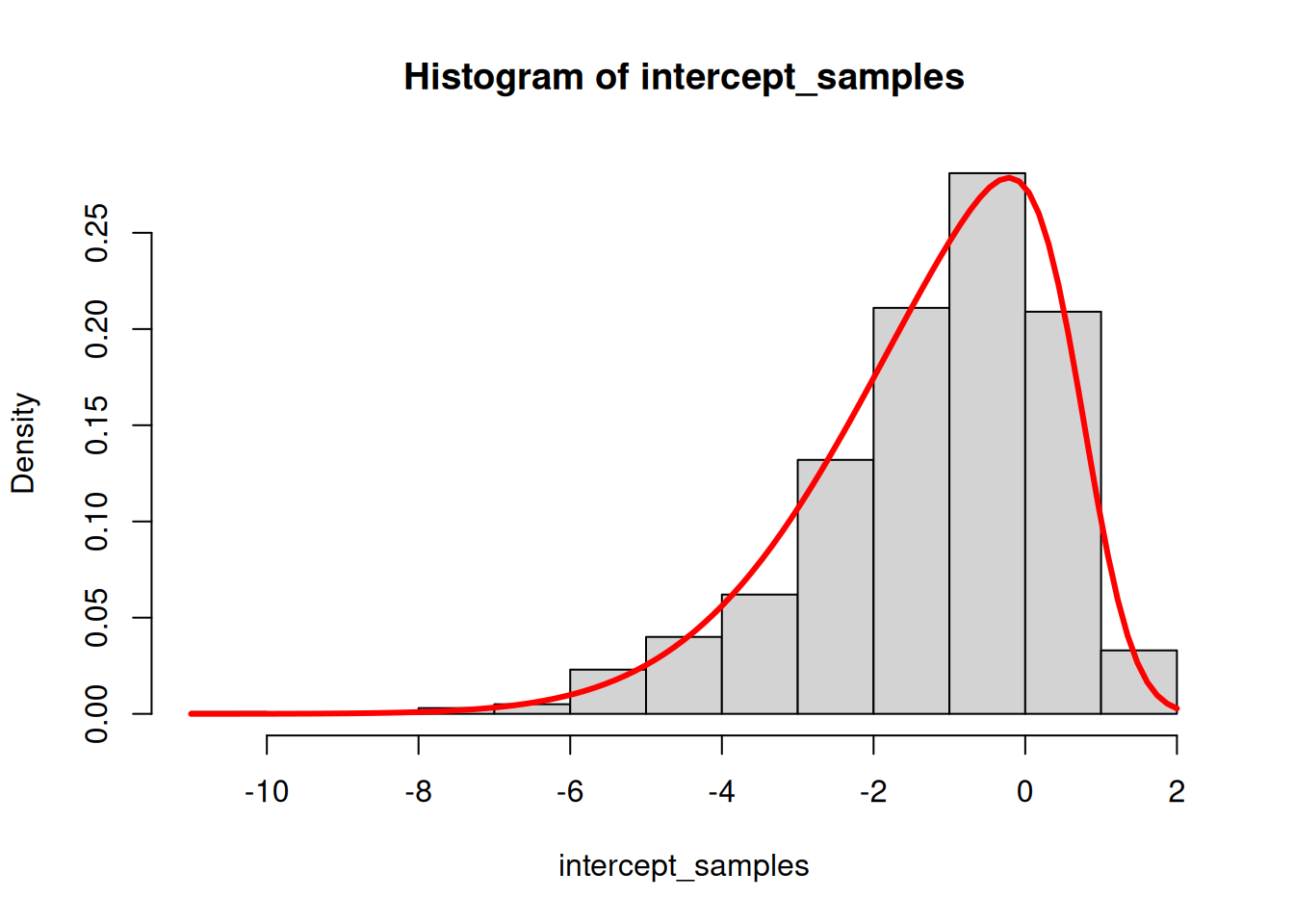
The remaining challenge is that in jmpost we specified a Gamma prior for \(\lambda\) which is now here the exponentiated intercept parameter. So in principle, we would need an ExpGamma prior on the intercept, meaning that if we exponentiate the intercept, it has a gamma distribution. However, this would again require a custom distribution. Let’s try to go with an approximation: we can just draw samples from the ExpGamma distribution (by sampling from a gamma distribution and taking the log) and then approximate this with a skewed normal distribution (see here for the Stan documentation):

set.seed(123)
intercept_samples <- log(rgamma(1000, 0.7, 1))

library(sn)
fit <- selm(intercept_samples ~ 1, family = "SN")
xi <- coef(fit, "DP")[1]
omega <- coef(fit, "DP")[2]
alpha <- coef(fit, "DP")[3]

hist(intercept_samples, probability = TRUE)
curve(dsn(x, xi, omega, alpha), add = TRUE, col = "red", lwd = 3)

The skew normal density curve approximates the histogram of the log gamma samples well.

Now we can finally specify the priors:

priors <- c(
    set_prior(
        glue::glue("skew_normal({xi}, {omega}, {alpha})"),
        class = "b",
        coef = "ones"
    ),
    prior(normal(0, 20), class = "b"),
    prior(gamma(0.7, 1), class = "alpha")
)

Let’s do a final check of the Stan code:

stancode(
    formula,
    data = os_data_with_log_kg_design,
    prior = priors,
    stanvars = sv_weibull_ph,
    family = family_weibull_ph()
)

// generated with brms 2.23.0
functions {
  
real weibull_ph_lpdf(real y, real mu, real alpha) {
  // real sigma = pow(1 / mu, 1 / alpha);
  real sigma = pow(mu, -1 * inv( alpha ));
  return weibull_lpdf(y | alpha, sigma);
}
real weibull_ph_lccdf(real y, real mu, real alpha) {
  real sigma = pow(mu, -1 * inv( alpha ));
  return weibull_lccdf(y | alpha, sigma);
}
real weibull_ph_lcdf(real y, real mu, real alpha) {
  real sigma = pow(mu, -1 * inv( alpha ));
  return weibull_lcdf(y | alpha, sigma);
}
real weibull_ph_rng(real mu, real alpha) {
  real sigma = pow(mu, -1 * inv( alpha ));
  return weibull_rng(alpha, sigma);
}

}
data {
  int<lower=1> N;  // total number of observations
  vector[N] Y;  // response variable
  // censoring indicator: 0 = event, 1 = right, -1 = left, 2 = interval censored
  array[N] int<lower=-1,upper=2> cens;
  int<lower=1> K;  // number of population-level effects
  matrix[N, K] X;  // population-level design matrix
  int prior_only;  // should the likelihood be ignored?
}
transformed data {
  // indices of censored data
  int Nevent = 0;
  int Nrcens = 0;
  int Nlcens = 0;
  array[N] int Jevent;
  array[N] int Jrcens;
  array[N] int Jlcens;
  // collect indices of censored data
  for (n in 1:N) {
    if (cens[n] == 0) {
      Nevent += 1;
      Jevent[Nevent] = n;
    } else if (cens[n] == 1) {
      Nrcens += 1;
      Jrcens[Nrcens] = n;
    } else if (cens[n] == -1) {
      Nlcens += 1;
      Jlcens[Nlcens] = n;
    }
  }
}
parameters {
  vector[K] b;  // regression coefficients
  real<lower=0> alpha;  // skewness parameter
}
transformed parameters {
  // prior contributions to the log posterior
  real lprior = 0;
  lprior += skew_normal_lpdf(b[1] | 0.758392879263355, 2.57341668661882, -4.8061893638208);
  lprior += normal_lpdf(b[2] | 0, 20);
  lprior += normal_lpdf(b[3] | 0, 20);
  lprior += normal_lpdf(b[4] | 0, 20);
  lprior += normal_lpdf(b[5] | 0, 20);
  lprior += normal_lpdf(b[6] | 0, 20);
  lprior += normal_lpdf(b[7] | 0, 20);
  lprior += gamma_lpdf(alpha | 0.7, 1);
}
model {
  // likelihood including constants
  if (!prior_only) {
    // initialize linear predictor term
    vector[N] mu = rep_vector(0.0, N);
    mu += X * b;
    mu = exp(mu);
    for (n in 1:N) {
      // special treatment of censored data
      if (cens[n] == 0) {
        target += weibull_ph_lpdf(Y[n] | mu[n], alpha);
      } else if (cens[n] == 1) {
        target += weibull_ph_lccdf(Y[n] | mu[n], alpha);
      } else if (cens[n] == -1) {
        target += weibull_ph_lcdf(Y[n] | mu[n], alpha);
      }
    }
  }
  // priors including constants
  target += lprior;
}
generated quantities {
}

Now we can fit the model:

save_file <- here("session-os/brms1.rds")
if (file.exists(save_file)) {
    fit <- readRDS(save_file)
} else {
    fit <- brm(
        formula = formula,
        data = os_data_with_log_kg_design,
        prior = priors,
        stanvars = sv_weibull_ph,
        family = family_weibull_ph(),
        chains = CHAINS,
        iter = ITER + WARMUP,
        warmup = WARMUP,
        seed = BAYES.SEED,
        refresh = REFRESH
    )
    saveRDS(fit, save_file)
}

summary(fit)

 Family: weibull_ph 
  Links: mu = log 
Formula: os_time | cens(os_cens) ~ 0 + ones + ecog1 + age + raceOTHER + raceWHITE + sexM + log_kg_est 
   Data: os_data_with_log_kg_design (Number of observations: 203) 
  Draws: 4 chains, each with iter = 3000; warmup = 2000; thin = 1;
         total post-warmup draws = 4000

Regression Coefficients:
           Estimate Est.Error l-95% CI u-95% CI Rhat Bulk_ESS Tail_ESS
ones          -1.59      0.63    -2.85    -0.38 1.00     1935     2531
ecog1          0.71      0.21     0.29     1.13 1.00     3317     2840
age            0.00      0.01    -0.01     0.02 1.00     1953     2532
raceOTHER      0.54      0.40    -0.30     1.27 1.00     3071     2139
raceWHITE     -0.03      0.23    -0.46     0.42 1.00     3052     2735
sexM           0.31      0.20    -0.07     0.69 1.00     3740     2938
log_kg_est     0.59      0.17     0.25     0.94 1.00     3821     3144

Further Distributional Parameters:
      Estimate Est.Error l-95% CI u-95% CI Rhat Bulk_ESS Tail_ESS
alpha     1.68      0.14     1.42     1.96 1.00     4072     2992

Draws were sampled using sample(hmc). For each parameter, Bulk_ESS
and Tail_ESS are effective sample size measures, and Rhat is the potential
scale reduction factor on split chains (at convergence, Rhat = 1).

So the model converged fast and well.

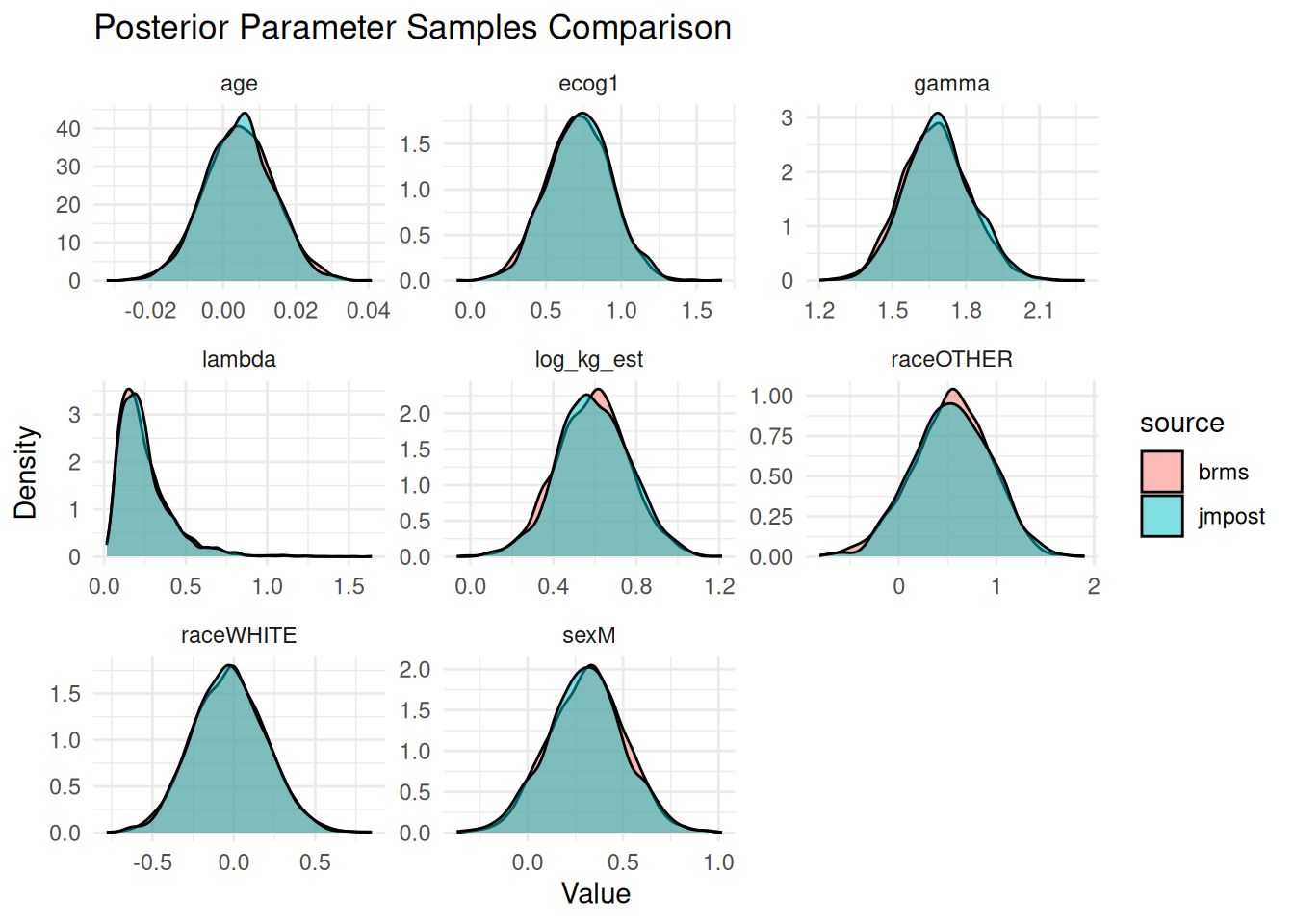
Comparison of results

Let’s compare the results of the brms model with the jmpost model.

First we load again the jmpost results:

draws_jmpost <- readRDS(here("session-os/os_draws.rds")) |>
    rename_variables(
        "gamma" = "sm_weibull_ph_gamma",
        "lambda" = "sm_weibull_ph_lambda"
    )
summary(draws_jmpost)

# A tibble: 8 × 10
  variable       mean   median      sd     mad      q5    q95  rhat ess_bulk
  <chr>         <dbl>    <dbl>   <dbl>   <dbl>   <dbl>  <dbl> <dbl>    <dbl>
1 ecog1       0.724    0.728   0.207   0.214    0.386  1.06   1.00      957.
2 age         0.00445  0.00463 0.00920 0.00937 -0.0101 0.0194 0.999    1043.
3 raceOTHER   0.542    0.542   0.400   0.419   -0.124  1.17   0.998     942.
4 raceWHITE  -0.0268  -0.0307  0.221   0.221   -0.373  0.333  1.00     1046.
5 sexM        0.302    0.303   0.201   0.198   -0.0342 0.630  1.00      718.
6 log_kg_est  0.597    0.587   0.172   0.170    0.321  0.880  1.00      742.
7 gamma       1.69     1.68    0.135   0.131    1.47   1.92   1.00      933.
8 lambda      0.248    0.208   0.164   0.115    0.0720 0.556  0.999     983.
# ℹ 1 more variable: ess_tail <dbl>

We prepare above brms results in the same format:

draws_brms <- as_draws_array(fit) |>
    mutate_variables(lambda = exp(b_ones)) |>
    rename_variables(
        "gamma" = "alpha",
        "ecog1" = "b_ecog1",
        "age" = "b_age",
        "raceOTHER" = "b_raceOTHER",
        "raceWHITE" = "b_raceWHITE",
        "sexM" = "b_sexM",
        "log_kg_est" = "b_log_kg_est"
    ) |>
    subset_draws(
        variable = c(
            "ecog1",
            "age",
            "raceOTHER",
            "raceWHITE",
            "sexM",
            "log_kg_est",
            "gamma",
            "lambda"
        )
    )
summary(draws_brms)

# A tibble: 8 × 10
  variable       mean   median      sd     mad      q5    q95  rhat ess_bulk
  <chr>         <dbl>    <dbl>   <dbl>   <dbl>   <dbl>  <dbl> <dbl>    <dbl>
1 ecog1       0.713    0.713   0.215   0.217    0.362  1.06   1.00     3317.
2 age         0.00459  0.00455 0.00964 0.00952 -0.0112 0.0205 1.00     1953.
3 raceOTHER   0.537    0.550   0.400   0.394   -0.155  1.16   1.00     3071.
4 raceWHITE  -0.0259  -0.0250  0.226   0.228   -0.389  0.353  1.00     3052.
5 sexM        0.312    0.317   0.199   0.200   -0.0149 0.631  1.00     3740.
6 log_kg_est  0.589    0.593   0.174   0.172    0.310  0.874  1.00     3821.
7 gamma       1.68     1.67    0.140   0.139    1.45   1.91   1.000    4072.
8 lambda      0.249    0.206   0.170   0.125    0.0719 0.565  1.00     1935.
# ℹ 1 more variable: ess_tail <dbl>

So the results agree well. We can also see this in density plots:

# Combine the draws into one data frame
draws_combined <- bind_rows(
    mutate(as_draws_df(draws_jmpost), source = "jmpost"),
    mutate(as_draws_df(draws_brms), source = "brms")
) |>
    select(-.chain, -.iteration, -.draw)

Warning: Dropping 'draws_df' class as required metadata was removed.

# Convert to long format for ggplot2
draws_long <- pivot_longer(
    draws_combined,
    cols = -source,
    names_to = "parameter",
    values_to = "value"
)

# Plot the densities
ggplot(draws_long, aes(x = value, fill = source)) +
    geom_density(alpha = 0.5) +
    facet_wrap(~parameter, scales = "free") +
    theme_minimal() +
    labs(
        title = "Posterior Parameter Samples Comparison",
        x = "Value",
        y = "Density"
    )

Generally these agree very well with each other. Overall we can expect a slight difference between the two results, because for the \(\lambda\) parameter we only approximately used the same prior distribution in brms compared to jmpost.