2. TGI model minimal workflow with `jmpost`

Authors

Daniel Sabanés Bové

Francois Mercier

Published

2025-02-12

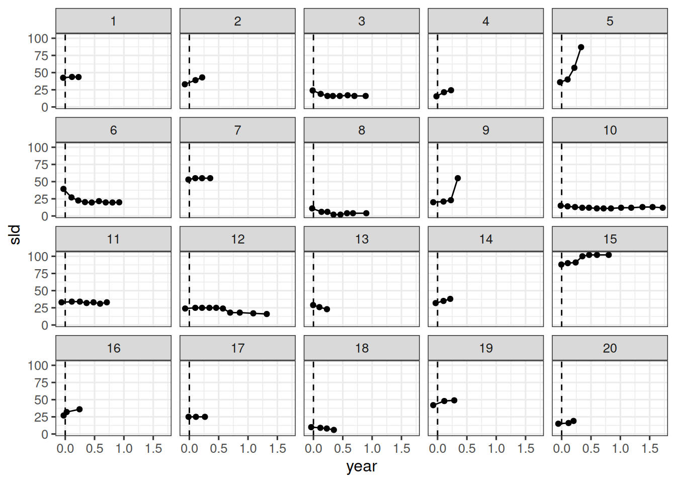
Let’s try to fit the same model now with jmpost. We will use the same data as in the previous notebook.

Setup and load data

First we need to load the necessary packages and set some default options for the MCMC sampling. We also set the theme for the plots to theme_bw with a base size of 12.

Show the code

library(bayesplot)
library(brms)
library(ggplot2)
library(gt)
library(here)
library(janitor)
library(jmpost)
library(modelr)
library(posterior)
library(readxl)
library(rstan)
library(tidybayes)
library(tidyverse)
library(truncnorm)

if (require(cmdstanr)) {
  # If cmdstanr is available, instruct brms to use cmdstanr as backend 
  # and cache all Stan binaries
  options(brms.backend = "cmdstanr", cmdstanr_write_stan_file_dir = here("_brms-cache"))
  dir.create(here("_brms-cache"), FALSE) # create cache directory if not yet available
} else {
  rstan::rstan_options(auto_write = TRUE)
}

# MCMC options
options(mc.cores = 4)
ITER <- 1000 # number of sampling iterations after warm up
WARMUP <- 2000 # number of warm up iterations
CHAINS <- 4
BAYES.SEED <- 878
REFRESH <- 500

theme_set(theme_bw(base_size = 12))

We also need a small function definition, which is still missing in brms:

Show the code

int_step <- function(x) {
  stopifnot(is.logical(x))
  ifelse(x, 1, 0)
}

We will use the publicly published tumor size data from the OAK study, see here. In particular we are using the S1 data set, which is the fully anonymized data set used in the publication. For simplicity, we have copied the data set in this GitHub repository.

Show the code

file_path <- here("data/journal.pcbi.1009822.s006.xlsx")

read_one_sheet <- function(sheet) {
    read_excel(file_path, sheet = sheet) |> 
    clean_names() |> 
    mutate(
        id = factor(as.character(patient_anonmyized)),
        day = as.integer(treatment_day),
        year = day / 365.25,
        target_lesion_long_diam_mm = case_match(
            target_lesion_long_diam_mm,
            "TOO SMALL TO MEASURE" ~ "2",
            "NOT EVALUABLE" ~ NA_character_,
            .default = target_lesion_long_diam_mm
        ),
        sld = as.numeric(target_lesion_long_diam_mm),
        sld = ifelse(sld == 0, 2, sld),
        study = factor(gsub("^Study_(\\d+)_Arm_\\d+$", "\\1", study_arm)),
        arm = factor(gsub("^Study_\\d+_Arm_(\\d+)$", "\\1", study_arm))
    ) |> 
    select(id, year, sld, study, arm)
}

tumor_data <- excel_sheets(file_path) |> 
    map(read_one_sheet) |> 
    bind_rows()

head(tumor_data)

# A tibble: 6 × 5
  id                      year   sld study arm  
  <fct>                  <dbl> <dbl> <fct> <fct>
1 3657015667902160896 -0.00548    33 1     1    
2 3657015667902160896  0.101      33 1     1    
3 3657015667902160896  0.230      32 1     1    
4 3657015667902160896  0.342      37 1     1    
5 3657015667902160896  0.446      49 1     1    
6 2080619628198763008 -0.00548    12 1     1

Show the code

summary(tumor_data)

                    id            year              sld        study   
 4308512445673410048 :  18   Min.   :-0.1314   Min.   :  2.0   1: 456  
 -4902532987801034752:  17   1st Qu.: 0.1123   1st Qu.: 17.0   2: 966  
 5394902984416364544 :  16   Median : 0.2847   Median : 30.0   3:2177  
 7160320731596789760 :  16   Mean   : 0.3822   Mean   : 36.1   4:4126  
 -4159496062492130816:  15   3rd Qu.: 0.5722   3rd Qu.: 49.0   5: 835  
 -7900338178541499392:  15   Max.   : 2.0753   Max.   :228.0           
 (Other)             :8463   NA's   :1         NA's   :69              
 arm     
 1:3108  
 2:3715  
 3: 291  
 4: 608  
 5: 227  
 6: 611

For simplicity, we will for now just use study 4 (this is the OAK study), and we rename the patient IDs:

Show the code

df <- tumor_data |> 
  filter(study == "4") |> 
  na.omit() |>
  droplevels() |> 
  mutate(id = factor(as.numeric(id)))

Here we have 701 patients. It is always a good idea to make a plot of the data. Let’s look at the first 20 patients e.g.:

Show the code

df |> 
  filter(as.integer(id) <= 20) |>
  ggplot(aes(x = year, y = sld, group = id)) +
  geom_line() +
  geom_point() +
  facet_wrap(~ id) +
  geom_vline(xintercept = 0, linetype = "dashed") +
  theme(legend.position = "none")

Data preparation

We start with the subject level data set. For the beginning, we want to treat all observations as if they come from a single arm and single study for now. Therefore we insert constant study and arm values here.

Show the code

subj_df <- data.frame(
  id = unique(df$id),
  arm = "arm",
  study = "study"
)
subj_data <- DataSubject(
  data = subj_df,
  subject = "id",
  arm = "arm",
  study = "study"
)

Next we prepare the longitudinal data object.

Show the code

long_df <- df |>
  select(id, year, sld)
long_data <- DataLongitudinal(
  data = long_df,
  formula = sld ~ year
)

Now we can create the JointData object:

Show the code

joint_data <- DataJoint(
    subject = subj_data,
    longitudinal = long_data
)

Model specification

The statistical model is specified in the jmpost vignette here.

Here we just want to fit the longitudinal data, therefore:

Show the code

tgi_mod <- JointModel(
    longitudinal = LongitudinalSteinFojo(
        mu_bsld = prior_normal(log(65), 1),
        mu_ks = prior_normal(log(0.52), 1),
        mu_kg = prior_normal(log(1.04), 1),
        omega_bsld = prior_normal(0, 3) |> set_limits(0, Inf),
        omega_ks = prior_normal(0, 3) |> set_limits(0, Inf),
        omega_kg = prior_normal(0, 3) |> set_limits(0, Inf),
        sigma = prior_normal(0, 3) |> set_limits(0, Inf)
    )
)

Note that the priors on the standard deviations, omega_* and sigma, are truncated to the positive domain. So we used here truncated normal priors.

Fit model

We can now fit the model using jmpost.

Show the code

save_file <- here("session-tgi/jm5.RData")
if (file.exists(save_file)) {
  load(save_file)
} else {
  mcmc_results <- sampleStanModel(
      tgi_mod,
      data = joint_data,
      iter_sampling = ITER,
      iter_warmup = WARMUP,
      chains = CHAINS,
      parallel_chains = CHAINS,
      thin = CHAINS,
      seed = BAYES.SEED,
      refresh = REFRESH
  )
  save(mcmc_results, file = save_file)
}

Let’s check the convergence of the population parameters:

Show the code

vars <- c(
    "lm_sf_mu_bsld",
    "lm_sf_mu_ks",
    "lm_sf_mu_kg",
    "lm_sf_sigma",
    "lm_sf_omega_bsld",
    "lm_sf_omega_ks",
    "lm_sf_omega_kg"
)

save_overall_file <- here("session-tgi/jm5_more.RData")
if (file.exists(save_overall_file)) {
  load(save_overall_file)
} else {
  mcmc_res_cmdstan <- cmdstanr::as.CmdStanMCMC(mcmc_results)
  mcmc_res_sum <- mcmc_res_cmdstan$summary(vars)
  vars_draws <- mcmc_res_cmdstan$draws(vars)
  loo_res <- mcmc_res_cmdstan$loo(r_eff = FALSE)
  save(mcmc_res_sum, vars_draws, loo_res, file = save_overall_file)
}
mcmc_res_sum

# A tibble: 7 × 10
  variable     mean median      sd     mad     q5    q95  rhat ess_bulk ess_tail
  <chr>       <dbl>  <dbl>   <dbl>   <dbl>  <dbl>  <dbl> <dbl>    <dbl>    <dbl>
1 lm_sf_mu_…  3.61   3.61  0.0236  0.0232   3.57   3.65   1.02     142.     188.
2 lm_sf_mu_… -1.27  -1.27  0.160   0.152   -1.54  -1.03   1.01     352.     500.
3 lm_sf_mu_… -1.35  -1.35  0.0828  0.0789  -1.49  -1.22   1.00     230.     456.
4 lm_sf_sig…  0.161  0.161 0.00233 0.00244  0.158  0.165  1.00     513.     875.
5 lm_sf_ome…  0.579  0.578 0.0156  0.0153   0.555  0.608  1.00     341.     576.
6 lm_sf_ome…  1.62   1.62  0.117   0.112    1.45   1.82   1.01     321.     509.
7 lm_sf_ome…  0.997  0.993 0.0505  0.0503   0.920  1.08   1.00     390.     595.

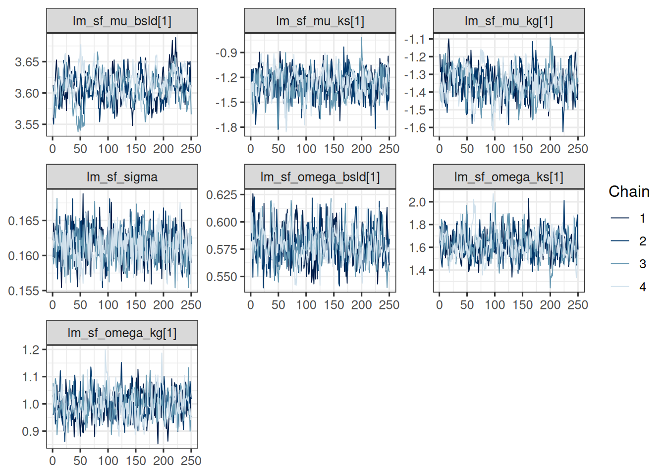
This looks good, let’s check the traceplots:

Show the code

# vars_draws <- mcmc_res_cmdstan$draws(vars)
mcmc_trace(vars_draws)

They also look ok, all chains are mixing well in the same range of parameter values.

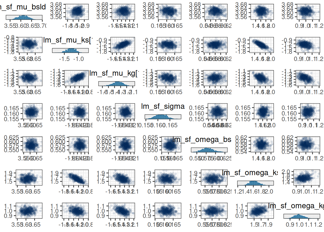
Also here we could look at the pairs plot:

Show the code

mcmc_pairs(
  vars_draws,
  off_diag_args = list(size = 1, alpha = 0.1)
)

Observation vs. model fit

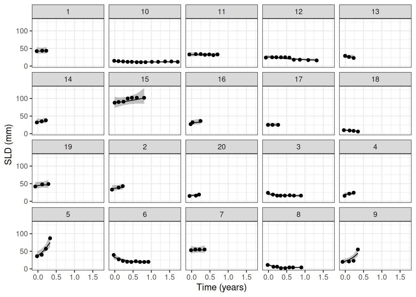
Let’s check the fit of the model to the data:

Show the code

pt_subset <- as.character(1:20)

save_fit_file <- here("session-tgi/jm5_fit.RData")
if (file.exists(save_fit_file)) {
  load(save_fit_file)
} else {
  fit_subset <- LongitudinalQuantities(
    mcmc_results, 
    grid = GridObserved(subjects = pt_subset)
  )
  save(fit_subset, file = save_fit_file)
}

autoplot(fit_subset)+
  labs(x = "Time (years)", y = "SLD (mm)")

So this works very nicely.

Prior vs. posterior

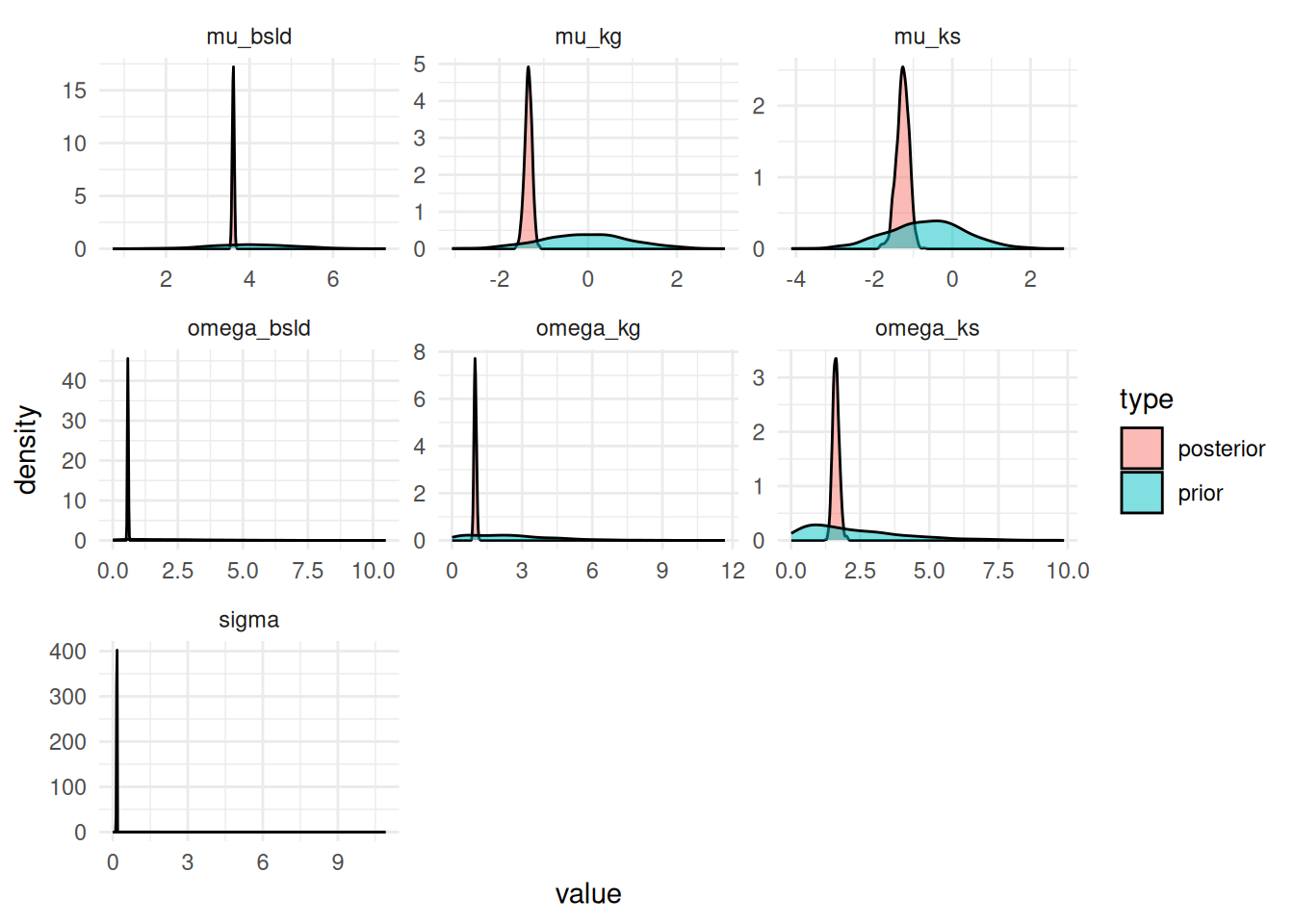
Let’s check the prior vs. posterior for the parameters:

Show the code

post_samples <- as_draws_df(vars_draws) |> 
  rename(
    mu_bsld = "lm_sf_mu_bsld[1]",
    mu_ks = "lm_sf_mu_ks[1]",
    mu_kg = "lm_sf_mu_kg[1]",
    omega_bsld = "lm_sf_omega_bsld[1]",
    omega_ks = "lm_sf_omega_ks[1]",
    omega_kg = "lm_sf_omega_kg[1]",
    sigma = lm_sf_sigma
  ) |> 
  mutate(type = "posterior") |> 
  select(mu_bsld, mu_ks, mu_kg, omega_bsld, omega_ks, omega_kg, sigma, type)

Warning: Dropping 'draws_df' class as required metadata was removed.

Show the code

n_prior_samples <- nrow(post_samples)
prior_samples <- data.frame(
    mu_bsld = rnorm(n_prior_samples, log(65), 1),
    mu_ks = rnorm(n_prior_samples, log(0.52), 1),
    mu_kg = rnorm(n_prior_samples, log(1.04), 1),
    omega_bsld = rtruncnorm(n_prior_samples, a = 0, mean = 0, sd = 3),
    omega_ks = rtruncnorm(n_prior_samples, a = 0, mean = 0, sd = 3),
    omega_kg = rtruncnorm(n_prior_samples, a = 0, mean = 0, sd = 3),
    sigma = rtruncnorm(n_prior_samples, a = 0, mean = 0, sd = 3)
  ) |> 
  mutate(type = "prior")

# Combine the two
combined_samples <- rbind(post_samples, prior_samples) |> 
  pivot_longer(cols = -type, names_to = "parameter", values_to = "value")

ggplot(combined_samples, aes(x = value, fill = type)) +
  geom_density(alpha = 0.5) +
  facet_wrap(~parameter, scales = "free") +
  theme_minimal()

This looks good, because the priors are covering the range of the posterior samples and are not too informative.

Parameter estimates

Here we need again to be careful: We are interested in the posterior mean estimates of the baseline, shrinkage and growth population rates on the original scale. Because we model them on the log scale as normal distributed, we need to use the mean of the log-normal distribution to get the mean on the original scale.

Show the code

post_sum <- post_samples |>
  mutate(
    theta_b0 = exp(mu_bsld + omega_bsld^2 / 2), 
    theta_ks = exp(mu_ks + omega_ks^2 / 2), 
    theta_kg = exp(mu_kg + omega_kg^2 / 2),
    cv_0 = sqrt(exp(omega_bsld^2) - 1),
    cv_s = sqrt(exp(omega_ks^2) - 1),
    cv_g = sqrt(exp(omega_kg^2) - 1)
  ) |>
  select(theta_b0, theta_ks, theta_kg, omega_bsld, omega_ks, omega_kg, cv_0, cv_s, cv_g, sigma) |>
  summarize_draws() |>
  gt() |>
  fmt_number(n_sigfig = 3)
post_sum

variable	mean	median	sd	mad	q5	q95	rhat	ess_bulk	ess_tail
theta_b0	43.7	43.8	1.10	1.12	42.0	45.5	1.00	151	201
theta_ks	1.06	1.05	0.129	0.120	0.871	1.30	1.00	226	408
theta_kg	0.428	0.427	0.0311	0.0306	0.378	0.479	1.00	318	472
omega_bsld	0.579	0.578	0.0156	0.0153	0.555	0.608	1.00	346	545
omega_ks	1.62	1.62	0.117	0.112	1.45	1.82	1.00	318	494
omega_kg	0.997	0.993	0.0505	0.0503	0.920	1.08	1.00	390	576
cv_0	0.631	0.630	0.0200	0.0196	0.600	0.668	1.00	346	545
cv_s	3.70	3.57	0.818	0.685	2.66	5.16	1.00	318	494
cv_g	1.31	1.30	0.106	0.103	1.15	1.49	1.00	390	576
sigma	0.161	0.161	0.00233	0.00244	0.158	0.165	1.00	495	844

We can see that these are consistent with the estimates from the brms model earlier.

Separate arm estimates

While there is no general covariates support in jmpost for the longitudinal models as of now, we can obtain separate estimates for the longitudinal model parameters: As detailed in the model specification here, as soon as we have the arm defined, then separate estimates for the arm-specific shrinkage and growth parameters will be obtained: Both the population means and standard deviation parameters are here arm-specific. (Note that this is slightly different from brms where we assumed earlier the same standard deviation independent of the treatment arm.)

So we need to define the subject data accordingly now with the arm information:

Show the code

subj_df_by_arm <- df |>
  select(id, arm) |>
  distinct() |> 
  mutate(study = "study")

subj_data_by_arm <- DataSubject(
  data = subj_df_by_arm,
  subject = "id",
  arm = "arm",
  study = "study"
)

We redefine the JointData object and can then fit the model, because the prior specification does not need to change: We assume iid priors on the arm-specific parameters here.

Show the code

joint_data_by_arm <- DataJoint(
    subject = subj_data_by_arm,
    longitudinal = long_data
)

Show the code

save_file <- here("session-tgi/jm6.RData")
if (file.exists(save_file)) {
  load(save_file)
} else {
  mcmc_results_by_arm <- sampleStanModel(
      tgi_mod,
      data = joint_data_by_arm,
      iter_sampling = ITER,
      iter_warmup = WARMUP,
      chains = CHAINS,
      parallel_chains = CHAINS,
      thin = CHAINS,
      seed = BAYES.SEED,
      refresh = REFRESH
  )
  save(mcmc_results_by_arm, file = save_file)
}

Let’s again check the convergence:

Show the code

vars <- c(
    "lm_sf_mu_bsld",
    "lm_sf_mu_ks",
    "lm_sf_mu_kg",
    "lm_sf_sigma",
    "lm_sf_omega_bsld",
    "lm_sf_omega_ks",
    "lm_sf_omega_kg"
)

save_arm_file <- here("session-tgi/jm6_more.RData")
if (file.exists(save_arm_file)) {
  load(save_arm_file)
} else {
  mcmc_res_cmdstan_by_arm <- cmdstanr::as.CmdStanMCMC(mcmc_results_by_arm)
  mcmc_res_sum_by_arm <- mcmc_res_cmdstan_by_arm$summary(vars)
  vars_draws_by_arm <- mcmc_res_cmdstan_by_arm$draws(vars)
  loo_by_arm <- mcmc_res_cmdstan_by_arm$loo(r_eff = FALSE)
  save(mcmc_res_sum_by_arm, vars_draws_by_arm, loo_by_arm, file = save_arm_file)
}
mcmc_res_sum_by_arm

# A tibble: 11 × 10
   variable    mean median      sd     mad     q5    q95  rhat ess_bulk ess_tail
   <chr>      <dbl>  <dbl>   <dbl>   <dbl>  <dbl>  <dbl> <dbl>    <dbl>    <dbl>
 1 lm_sf_mu…  3.61   3.61  0.0211  0.0217   3.58   3.65  1.00      244.     502.
 2 lm_sf_mu… -0.752 -0.730 0.222   0.216   -1.14  -0.398 1.01      592.     673.
 3 lm_sf_mu… -1.52  -1.51  0.222   0.217   -1.90  -1.17  1.00      706.     850.
 4 lm_sf_mu… -1.11  -1.11  0.138   0.139   -1.35  -0.900 1.00      594.     814.
 5 lm_sf_mu… -1.35  -1.35  0.103   0.104   -1.52  -1.19  1.00      560.     776.
 6 lm_sf_si…  0.161  0.161 0.00224 0.00228  0.157  0.165 1.00      892.     941.
 7 lm_sf_om…  0.577  0.577 0.0159  0.0153   0.551  0.603 1.00      511.     672.
 8 lm_sf_om…  1.34   1.33  0.150   0.152    1.11   1.60  1.00      630.     844.
 9 lm_sf_om…  1.76   1.76  0.161   0.150    1.51   2.05  1.00      662.     990.
10 lm_sf_om…  0.765  0.758 0.0710  0.0685   0.662  0.891 0.999     809.     951.
11 lm_sf_om…  1.10   1.10  0.0705  0.0684   0.991  1.22  0.999     669.     736.

Let’s again tabulate the parameter estimates:

Show the code

post_samples_by_arm <- as_draws_df(vars_draws_by_arm) |> 
  rename(
    mu_bsld = "lm_sf_mu_bsld[1]",
    mu_ks1 = "lm_sf_mu_ks[1]",
    mu_ks2 = "lm_sf_mu_ks[2]",
    mu_kg1 = "lm_sf_mu_kg[1]",
    mu_kg2 = "lm_sf_mu_kg[2]",
    omega_bsld = "lm_sf_omega_bsld[1]",
    omega_ks1 = "lm_sf_omega_ks[1]",
    omega_ks2 = "lm_sf_omega_ks[2]",
    omega_kg1 = "lm_sf_omega_kg[1]",
    omega_kg2 = "lm_sf_omega_kg[2]",
    sigma = lm_sf_sigma
  ) |> 
  mutate(
    theta_b0 = exp(mu_bsld + omega_bsld^2 / 2), 
    theta_ks1 = exp(mu_ks1 + omega_ks1^2 / 2), 
    theta_ks2 = exp(mu_ks2 + omega_ks2^2 / 2),
    theta_kg1 = exp(mu_kg1 + omega_kg1^2 / 2),
    theta_kg2 = exp(mu_kg2 + omega_kg2^2 / 2),
    cv_0 = sqrt(exp(omega_bsld^2) - 1),
    cv_s1 = sqrt(exp(omega_ks1^2) - 1),
    cv_s2 = sqrt(exp(omega_ks2^2) - 1),
    cv_g1 = sqrt(exp(omega_kg1^2) - 1),
    cv_g2 = sqrt(exp(omega_kg2^2) - 1)
  ) 
  
post_sum_by_arm <- post_samples_by_arm |>
  select(
    theta_b0, theta_ks1, theta_ks2, theta_kg1, theta_kg2, 
    omega_bsld, omega_ks1, omega_ks2, omega_kg1, omega_kg2, 
    cv_0, cv_s1, cv_s2, cv_g1, cv_g2, sigma) |>
  summarize_draws() |>
  gt() |>
  fmt_number(n_sigfig = 3)

Warning: Dropping 'draws_df' class as required metadata was removed.

Show the code

post_sum_by_arm

variable	mean	median	sd	mad	q5	q95	rhat	ess_bulk	ess_tail
theta_b0	43.7	43.7	0.999	1.05	42.1	45.4	1.00	227	558
theta_ks1	1.18	1.17	0.152	0.146	0.961	1.44	1.00	530	696
theta_ks2	1.07	1.04	0.209	0.183	0.779	1.42	1.00	344	443
theta_kg1	0.444	0.443	0.0490	0.0489	0.365	0.527	1.00	539	712
theta_kg2	0.479	0.478	0.0487	0.0479	0.399	0.563	1.00	735	908
omega_bsld	0.577	0.577	0.0159	0.0153	0.551	0.603	1.00	504	659
omega_ks1	1.34	1.33	0.150	0.152	1.11	1.60	1.00	620	838
omega_ks2	1.76	1.76	0.161	0.150	1.51	2.05	1.00	651	972
omega_kg1	0.765	0.758	0.0710	0.0685	0.662	0.891	0.999	799	943
omega_kg2	1.10	1.10	0.0705	0.0684	0.991	1.22	1.00	649	693
cv_0	0.629	0.628	0.0205	0.0196	0.596	0.662	1.00	504	659
cv_s1	2.33	2.22	0.601	0.547	1.55	3.46	1.00	620	838
cv_s2	4.90	4.58	1.64	1.25	2.96	8.11	1.00	651	972
cv_g1	0.897	0.880	0.112	0.105	0.742	1.10	0.999	799	943
cv_g2	1.55	1.54	0.175	0.163	1.29	1.85	1.00	649	693
sigma	0.161	0.161	0.00224	0.00228	0.157	0.165	1.00	885	881

Here again the shrinkage rate in the treatment arm 1 seems higher than in the treatment arm 2. However, the difference is not as pronounced as in the brms model before with the same standard deviation for both arms. We can again calculate the posterior probability that the shrinkage rate in arm 1 is higher than in arm 2:

Show the code

prob_ks1_greater_ks2 <- mean(post_samples_by_arm$theta_ks1 > post_samples_by_arm$theta_ks2)
prob_ks1_greater_ks2

[1] 0.706

So the posterior probability is now only around 71%.

Model comparison with LOO

As we have seen for brms, also for jmpost we can easily compute the LOO criterion:

Show the code

# loo_res <- mcmc_res_cmdstan$loo(r_eff = FALSE)
loo_res


Computed from 1000 by 4099 log-likelihood matrix.

         Estimate    SE
elpd_loo -12957.3  95.8
p_loo      1137.1  38.4
looic     25914.5 191.6
------
MCSE of elpd_loo is NA.
MCSE and ESS estimates assume independent draws (r_eff=1).

Pareto k diagnostic values:
                          Count Pct.    Min. ESS
(-Inf, 0.67]   (good)     3665  89.4%   26      
   (0.67, 1]   (bad)       363   8.9%   <NA>    
    (1, Inf)   (very bad)   71   1.7%   <NA>    
See help('pareto-k-diagnostic') for details.

Underneath this is using the $loo() method from cmdstanr.

And we can compare this to the LOO of the model with separate arm estimates:

Show the code

# loo_by_arm <- mcmc_res_cmdstan_by_arm$loo(r_eff = FALSE)
loo_by_arm


Computed from 1000 by 4099 log-likelihood matrix.

         Estimate    SE
elpd_loo -12931.8  95.6
p_loo      1121.5  36.8
looic     25863.5 191.1
------
MCSE of elpd_loo is NA.
MCSE and ESS estimates assume independent draws (r_eff=1).

Pareto k diagnostic values:
                          Count Pct.    Min. ESS
(-Inf, 0.67]   (good)     3652  89.1%   48      
   (0.67, 1]   (bad)       374   9.1%   <NA>    
    (1, Inf)   (very bad)   73   1.8%   <NA>    
See help('pareto-k-diagnostic') for details.

So the model by treatment arm performs here better than the model without treatment arm specific growth and shrinkage parameters.

Tipps and tricks

Also here it is possible to look at the underlying Stan code:

Show the code

tmp <- tempfile()
write_stan(tgi_mod, destination = tmp)
file.edit(tmp) # opens the Stan file in the default editor

It is not trivial to transport saved models from one computer to another. This is because cmdstanr only loads the results it currently needs from disk into memory, and thus into the R session. If you want to transport the model to another computer, you need to save the Stan code and the data, and then re-run the model on the other computer. This is because the model object in R is only a reference to the model on disk, not the model itself. Note that there is the $save_object() method, see here, however this leads to very large files (here about 300 MB for one fit) and can thus not be uploaded to typical git repositories. Therefore above we saved interim result objects separately as needed.
It is important to explicitly define the truncation boundaries for the truncated normal priors, because otherwise the MCMC results will not be correct.