3. Generalized Stein-Fojo model

This appendix shows how the generalized Stein-Fojo model can be implemented in a Bayesian framework using the brms package in R.

Setup and load data

First we need to load the necessary packages and set some default options for the MCMC sampling. We also set the theme for the plots to theme_bw with a base size of 12.

library(bayesplot)
library(brms)
library(ggplot2)
library(gt)
library(here)
library(janitor)
library(jmpost)
library(modelr)
library(posterior)
library(readxl)
library(rstan)
library(tidybayes)
library(tidyverse)
library(truncnorm)

if (require(cmdstanr)) {
  # If cmdstanr is available, instruct brms to use cmdstanr as backend 
  # and cache all Stan binaries
  options(brms.backend = "cmdstanr", cmdstanr_write_stan_file_dir = here("_brms-cache"))
  dir.create(here("_brms-cache"), FALSE) # create cache directory if not yet available
} else {
  rstan::rstan_options(auto_write = TRUE)
}

# MCMC options
options(mc.cores = 4)
ITER <- 1000 # number of sampling iterations after warm up
WARMUP <- 2000 # number of warm up iterations
CHAINS <- 4
BAYES.SEED <- 878
REFRESH <- 500

theme_set(theme_bw(base_size = 12))

We also need a small function definition, which is still missing in brms:

int_step <- function(x) {
  stopifnot(is.logical(x))
  ifelse(x, 1, 0)
}

We will use the publicly published tumor size data from the OAK study, see here. In particular we are using the S1 data set, which is the fully anonymized data set used in the publication. For simplicity, we have copied the data set in this GitHub repository.

file_path <- here("data/journal.pcbi.1009822.s006.xlsx")

read_one_sheet <- function(sheet) {
    read_excel(file_path, sheet = sheet) |> 
    clean_names() |> 
    mutate(
        id = factor(as.character(patient_anonmyized)),
        day = as.integer(treatment_day),
        year = day / 365.25,
        target_lesion_long_diam_mm = case_match(
            target_lesion_long_diam_mm,
            "TOO SMALL TO MEASURE" ~ "2",
            "NOT EVALUABLE" ~ NA_character_,
            .default = target_lesion_long_diam_mm
        ),
        sld = as.numeric(target_lesion_long_diam_mm),
        sld = ifelse(sld == 0, 2, sld),
        study = factor(gsub("^Study_(\\d+)_Arm_\\d+$", "\\1", study_arm)),
        arm = factor(gsub("^Study_\\d+_Arm_(\\d+)$", "\\1", study_arm))
    ) |> 
    select(id, year, sld, study, arm)
}

tumor_data <- excel_sheets(file_path) |> 
    map(read_one_sheet) |> 
    bind_rows()

head(tumor_data)

# A tibble: 6 × 5
  id                      year   sld study arm  
  <fct>                  <dbl> <dbl> <fct> <fct>
1 3657015667902160896 -0.00548    33 1     1    
2 3657015667902160896  0.101      33 1     1    
3 3657015667902160896  0.230      32 1     1    
4 3657015667902160896  0.342      37 1     1    
5 3657015667902160896  0.446      49 1     1    
6 2080619628198763008 -0.00548    12 1     1    

summary(tumor_data)

                    id            year              sld        study   
 4308512445673410048 :  18   Min.   :-0.1314   Min.   :  2.0   1: 456  
 -4902532987801034752:  17   1st Qu.: 0.1123   1st Qu.: 17.0   2: 966  
 5394902984416364544 :  16   Median : 0.2847   Median : 30.0   3:2177  
 7160320731596789760 :  16   Mean   : 0.3822   Mean   : 36.1   4:4126  
 -4159496062492130816:  15   3rd Qu.: 0.5722   3rd Qu.: 49.0   5: 835  
 -7900338178541499392:  15   Max.   : 2.0753   Max.   :228.0           
 (Other)             :8463   NA's   :1         NA's   :69              
 arm     
 1:3108  
 2:3715  
 3: 291  
 4: 608  
 5: 227  
 6: 611  
         

For simplicity, we will for now just use study 4 (this is the OAK study), and we rename the patient IDs:

df <- tumor_data |> 
  filter(study == "4") |> 
  na.omit() |>
  droplevels() |> 
  mutate(id = factor(as.numeric(id)))

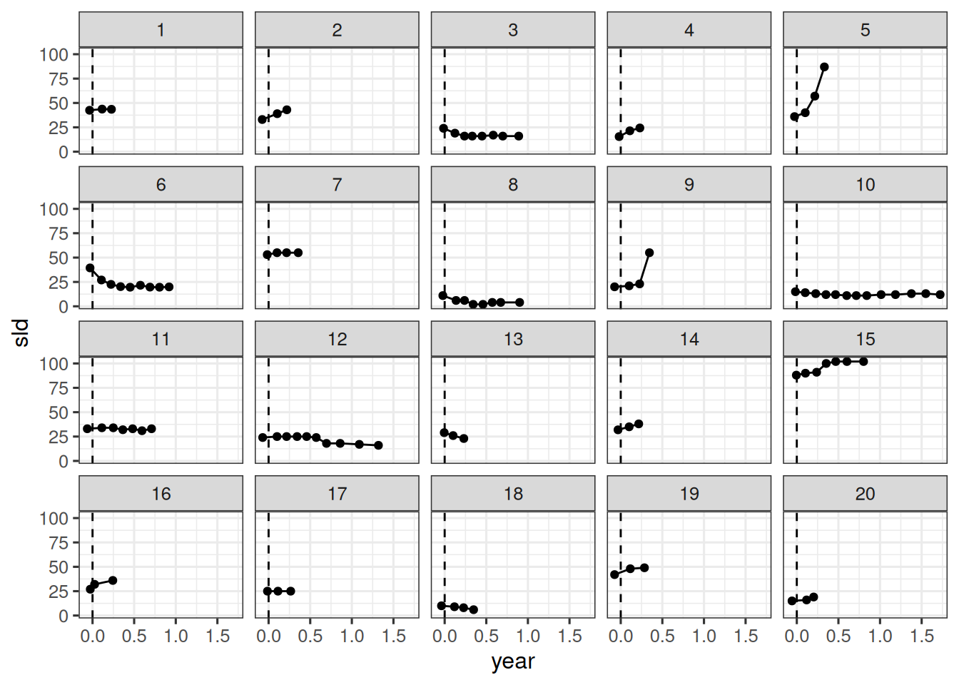
Here we have 701 patients. It is always a good idea to make a plot of the data. Let’s look at the first 20 patients e.g.:

df |> 
  filter(as.integer(id) <= 20) |>
  ggplot(aes(x = year, y = sld, group = id)) +
  geom_line() +
  geom_point() +
  facet_wrap(~ id) +
  geom_vline(xintercept = 0, linetype = "dashed") +
  theme(legend.position = "none")

Generalized Stein-Fojo model

Here we have an additional parameter \(\phi\), which is the weight for the shrinkage in the double exponential model. The model is then:

\[ y^{*}(t_{ij}) = \psi_{b_{0}i} \{ \psi_{\phi i} \exp(- \psi_{k_{s}i} \cdot t_{ij}) + (1 - \psi_{\phi i}) \exp(\psi_{k_{g}i} \cdot t_{ij}) \} \]

for positive times \(t_{ij}\). Again, if the time \(t\) is negative, i.e. the treatment has not started yet, then it is reasonable to assume that the tumor cannot shrink yet. That is, we have then \(\phi_i = 0\). Therefore, the final model for the mean SLD is:

\[ y^{*}(t_{ij}) = \begin{cases} \psi_{b_{0}i} \exp(\psi_{k_{g}i} \cdot t_{ij}) & \text{if } t_{ij} < 0 \\ \psi_{b_{0}i} \{ \psi_{\phi i} \exp(- \psi_{k_{s}i} \cdot t_{ij}) + (1 - \psi_{\phi i}) \exp(\psi_{k_{g}i} \cdot t_{ij}) \} & \text{if } t_{ij} \geq 0 \end{cases} \]

In terms of likelihood and priors, we can use the same assumptions as in the previous model. The only difference is that we have to model the \(\phi\) parameter. We can use a logit-normal distribution for this parameter. This is a normal distribution on the logit scale, which is then transformed to the unit interval. \[ \psi_{\phi i} \sim \text{LogitNormal}(\text{logit}(0.5) = 0, 0.5) \]

Fit model

We can now fit the model using brms. The structure is determined by the model formula:

formula <- bf(sld ~ ystar, nl = TRUE) +
  # Define the mean for the likelihood
  nlf(
    ystar ~ 
      int_step(year > 0) * 
        (b0 * (phi * exp(-ks * year) + (1 - phi) * exp(kg * year))) +
      int_step(year <= 0) * 
        (b0 * exp(kg * year))
  ) +
  # As before:
  nlf(sigma ~ log(tau) + log(ystar)) +
  lf(tau ~ 1) +
  # Define nonlinear parameter transformations:
  nlf(b0 ~ exp(lb0)) +
  nlf(phi ~ inv_logit(tphi)) +
  nlf(ks ~ exp(lks)) +
  nlf(kg ~ exp(lkg)) +
  # Define random effect structure:
  lf(lb0 ~ 1 + (1 | id)) + 
  lf(tphi ~ 1 + (1 | id)) + 
  lf(lks ~ 1 + (1 | id)) +
  lf(lkg ~ 1 + (1 | id))

# Define the priors
priors <- c(
  prior(normal(log(65), 1), nlpar = "lb0"),
  prior(normal(log(0.52), 0.1), nlpar = "lks"),
  prior(normal(log(1.04), 1), nlpar = "lkg"),
  prior(normal(0, 0.5), nlpar = "tphi"),
  prior(normal(0, 3), lb = 0, nlpar = "lb0", class = "sd"),
  prior(normal(0, 3), lb = 0, nlpar = "lks", class = "sd"),
  prior(normal(0, 3), lb = 0, nlpar = "lkg", class = "sd"),
  prior(student_t(3, 0, 22.2), lb = 0, nlpar = "tphi", class = "sd"),
  prior(normal(0, 3), lb = 0, nlpar = "tau")
)

# Initial values to avoid problems at the beginning
n_patients <- nlevels(df$id)
inits <- list(
  b_lb0 = array(3.61),
  b_lks = array(-1.25),
  b_lkg = array(-1.33),
  b_tphi = array(0),
  sd_1 = array(0.58),
  sd_2 = array(1.6),
  sd_3 = array(0.994),
  sd_4 = array(0.1),
  b_tau = array(0.161),
  z_1 = matrix(0, nrow = 1, ncol = n_patients),
  z_2 = matrix(0, nrow = 1, ncol = n_patients),
  z_3 = matrix(0, nrow = 1, ncol = n_patients),
  z_4 = matrix(0, nrow = 1, ncol = n_patients)
)

# Fit the model
save_file <- here("session-tgi/gsf1.RData")
if (file.exists(save_file)) {
  load(save_file)
} else {
  fit <- brm(
    formula = formula,
    data = df,
    prior = priors,
    family = gaussian(),
    init = rep(list(inits), CHAINS),
    chains = CHAINS, 
    iter = WARMUP + ITER, 
    warmup = WARMUP, 
    seed = BAYES.SEED,
    refresh = REFRESH
  )
  save(fit, file = save_file)
}

# Summarize the fit
summary(fit)

Warning: There were 41 divergent transitions after warmup. Increasing
adapt_delta above 0.8 may help. See
http://mc-stan.org/misc/warnings.html#divergent-transitions-after-warmup

 Family: gaussian 
  Links: mu = identity; sigma = log 
Formula: sld ~ eta 
         eta ~ int_step(year > 0) * (b0 * (phi * exp(-ks * year) + (1 - phi) * exp(kg * year))) + int_step(year <= 0) * (b0 * exp(kg * year))
         sigma ~ log(tau) + log(eta)
         tau ~ 1
         b0 ~ exp(lb0)
         phi ~ inv_logit(tphi)
         ks ~ exp(lks)
         kg ~ exp(lkg)
         lb0 ~ 1 + (1 | id)
         tphi ~ 1 + (1 | id)
         lks ~ 1 + (1 | id)
         lkg ~ 1 + (1 | id)
   Data: df (Number of observations: 4099) 
  Draws: 4 chains, each with iter = 3000; warmup = 2000; thin = 1;
         total post-warmup draws = 4000

Multilevel Hyperparameters:
~id (Number of levels: 701) 
                   Estimate Est.Error l-95% CI u-95% CI Rhat Bulk_ESS Tail_ESS
sd(lb0_Intercept)      0.58      0.02     0.55     0.61 1.01      382      606
sd(tphi_Intercept)     2.12      0.18     1.78     2.49 1.01      611     1216
sd(lks_Intercept)      2.16      0.14     1.90     2.46 1.00      520     1282
sd(lkg_Intercept)      1.18      0.09     1.01     1.36 1.00      899     1766

Regression Coefficients:
               Estimate Est.Error l-95% CI u-95% CI Rhat Bulk_ESS Tail_ESS
tau_Intercept      0.15      0.00     0.14     0.15 1.00     1611     2351
lb0_Intercept      3.63      0.02     3.59     3.68 1.03      221      547
tphi_Intercept    -0.14      0.22    -0.57     0.27 1.00      424      839
lks_Intercept     -0.62      0.10    -0.81    -0.43 1.00     1170     1868
lkg_Intercept     -1.15      0.14    -1.43    -0.89 1.00      699     1488

Draws were sampled using sample(hmc). For each parameter, Bulk_ESS
and Tail_ESS are effective sample size measures, and Rhat is the potential
scale reduction factor on split chains (at convergence, Rhat = 1).

In total this took 76 minutes on my laptop.

Parameter estimates

post_df <- as_draws_df(fit)
head(names(post_df), 10)

 [1] "b_tau_Intercept"        "b_lb0_Intercept"        "b_tphi_Intercept"      
 [4] "b_lks_Intercept"        "b_lkg_Intercept"        "sd_id__lb0_Intercept"  
 [7] "sd_id__tphi_Intercept"  "sd_id__lks_Intercept"   "sd_id__lkg_Intercept"  
[10] "r_id__lb0[1,Intercept]"

post_df <- post_df |>
  mutate(
    theta_b0 = exp(b_lb0_Intercept + sd_id__lb0_Intercept^2 / 2),
    theta_ks = exp(b_lks_Intercept + sd_id__lks_Intercept^2 / 2),
    theta_kg = exp(b_lkg_Intercept + sd_id__lkg_Intercept^2 / 2),
    theta_phi = plogis(b_tphi_Intercept),
    omega_0 = sd_id__lb0_Intercept,
    omega_s = sd_id__lks_Intercept,
    omega_g = sd_id__lkg_Intercept,
    omega_phi = sd_id__tphi_Intercept,
    cv_0 = sqrt(exp(sd_id__lb0_Intercept^2) - 1),
    cv_s = sqrt(exp(sd_id__lks_Intercept^2) - 1),
    cv_g = sqrt(exp(sd_id__lkg_Intercept^2) - 1),
    sigma = b_tau_Intercept
  )

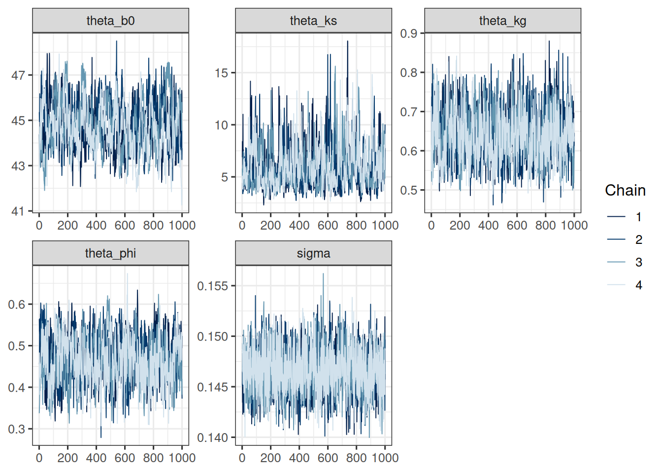
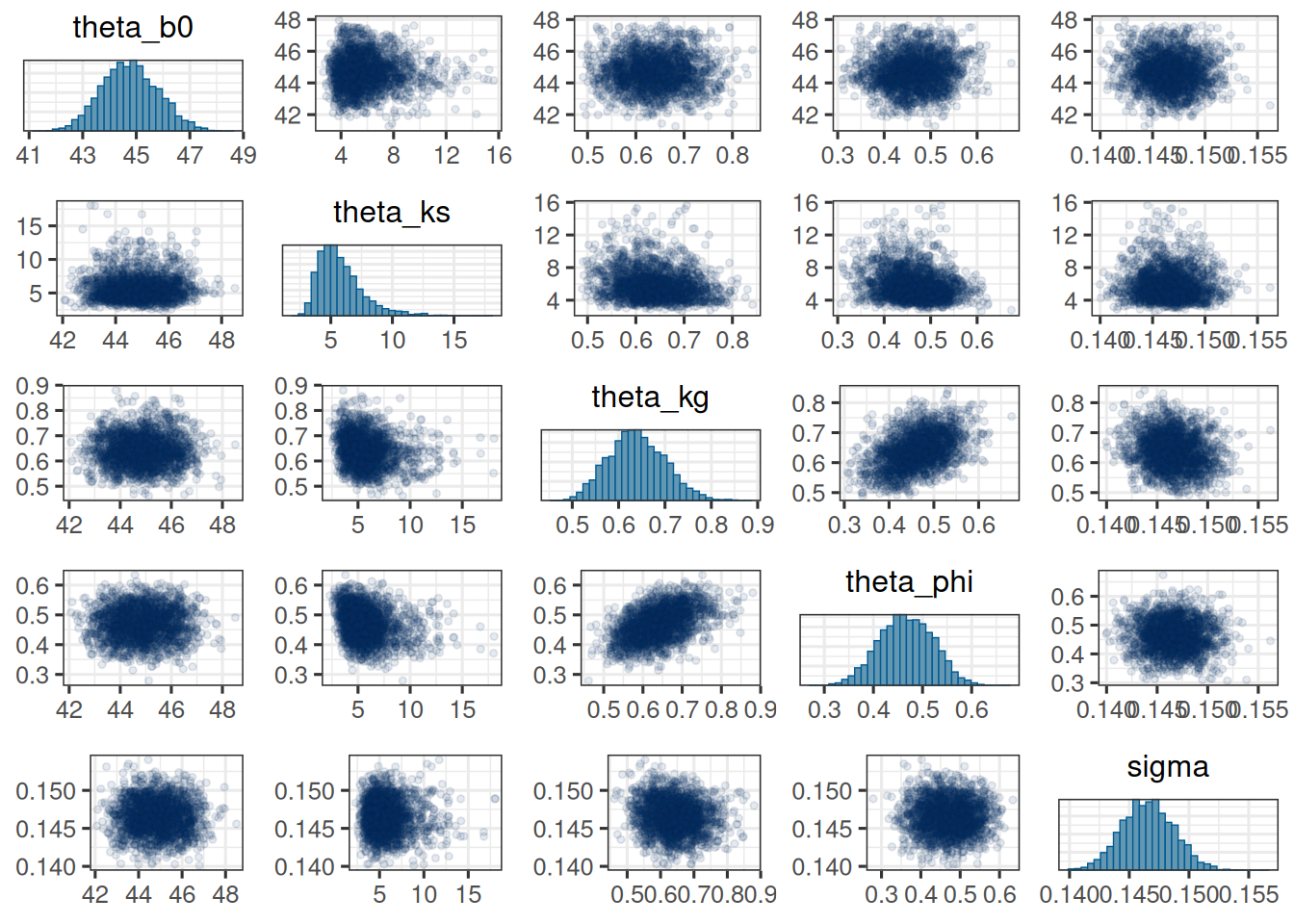
Let’s first look at the population level parameters:

gsf_pop_params <- c("theta_b0", "theta_ks", "theta_kg", "theta_phi", "sigma")

mcmc_trace(post_df, pars = gsf_pop_params)

mcmc_pairs(
  post_df, 
  pars = gsf_pop_params,
  off_diag_args = list(size = 1, alpha = 0.1)
)

The trace plots look good. The chains seem to have converged and the pairs plot shows no strong correlations between the parameters. Let’s check the table:

post_sum <- post_df |>
  select(theta_b0, theta_ks, theta_kg, theta_phi, omega_0, omega_s, omega_g, omega_phi, sigma) |>
  summarize_draws() |>
  gt() |>
  fmt_number(decimals = 3)

Warning: Dropping 'draws_df' class as required metadata was removed.

post_sum

variable	mean	median	sd	mad	q5	q95	rhat	ess_bulk	ess_tail
theta_b0	44.766	44.746	1.057	1.073	43.074	46.528	1.007	179.361	378.906
theta_ks	5.857	5.444	1.924	1.582	3.589	9.560	1.003	384.622	905.388
theta_kg	0.640	0.637	0.061	0.062	0.541	0.745	1.000	685.379	1,885.264
theta_phi	0.467	0.466	0.055	0.058	0.376	0.555	1.003	419.761	831.991
omega_0	0.578	0.578	0.016	0.017	0.553	0.606	1.001	376.483	628.807
omega_s	2.159	2.155	0.145	0.145	1.929	2.412	1.002	521.866	1,265.639
omega_g	1.177	1.174	0.090	0.090	1.037	1.333	1.002	868.075	1,746.640
omega_phi	2.117	2.108	0.182	0.184	1.833	2.423	1.003	603.806	1,215.066
sigma	0.147	0.147	0.002	0.002	0.143	0.150	1.000	1,575.916	2,168.010

So \(\theta_{\phi}\) is estimated around 0.5. The other parameters are similar to the previous Stein-Fojo model, but we see a larger \(\theta_{k_s}\) e.g.

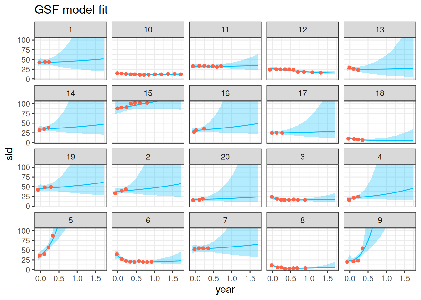
Observation vs model fit

We can now compare the model fit to the observations. Let’s do this for the first 20 patients again:

pt_subset <- as.character(1:20)
df_subset <- df |> 
  filter(id %in% pt_subset)

df_sim <- df_subset |> 
  data_grid(
    id = pt_subset, 
    year = seq_range(year, 101)
  ) |>
  add_epred_draws(fit) |>
  median_qi()

df_sim |>
  ggplot(aes(x = year, y = sld)) +
  facet_wrap(~ id) +
  geom_ribbon(
    aes(y = .epred, ymin = .lower, ymax = .upper), 
    alpha = 0.3, 
    fill = "deepskyblue"
  ) +
  geom_line(aes(y = .epred), color = "deepskyblue") +
  geom_point(data = df_subset, color = "tomato") +
  coord_cartesian(ylim = range(df_subset$sld)) +
  scale_fill_brewer(palette = "Greys") +
  labs(title = "GSF model fit")

This also looks good. The model seems to capture the data well.

With jmpost

This model can also be fit with the jmpost package. The corresponding function is LongitudinalGSF. The statistical model is specified in the vignette here.

Homework: Implement the generalized Stein-Fojo model with jmpost and compare the results with the brms implementation.