4. Claret-Bruno model

This appendix shows how the Claret-Bruno model can be implemented in a Bayesian framework using the brms package in R.

Setup and load data

First we need to load the necessary packages and set some default options for the MCMC sampling. We also set the theme for the plots to theme_bw with a base size of 12.

library(bayesplot)
library(brms)
library(ggplot2)
library(gt)
library(here)
library(janitor)
library(jmpost)
library(modelr)
library(posterior)
library(readxl)
library(rstan)
library(tidybayes)
library(tidyverse)
library(truncnorm)

if (require(cmdstanr)) {
  # If cmdstanr is available, instruct brms to use cmdstanr as backend 
  # and cache all Stan binaries
  options(brms.backend = "cmdstanr", cmdstanr_write_stan_file_dir = here("_brms-cache"))
  dir.create(here("_brms-cache"), FALSE) # create cache directory if not yet available
} else {
  rstan::rstan_options(auto_write = TRUE)
}

# MCMC options
options(mc.cores = 4)
ITER <- 1000 # number of sampling iterations after warm up
WARMUP <- 2000 # number of warm up iterations
CHAINS <- 4
BAYES.SEED <- 878
REFRESH <- 500

theme_set(theme_bw(base_size = 12))

We also need a small function definition, which is still missing in brms:

int_step <- function(x) {
  stopifnot(is.logical(x))
  ifelse(x, 1, 0)
}

We will use the publicly published tumor size data from the OAK study, see here. In particular we are using the S1 data set, which is the fully anonymized data set used in the publication. For simplicity, we have copied the data set in this GitHub repository.

file_path <- here("data/journal.pcbi.1009822.s006.xlsx")

read_one_sheet <- function(sheet) {
    read_excel(file_path, sheet = sheet) |> 
    clean_names() |> 
    mutate(
        id = factor(as.character(patient_anonmyized)),
        day = as.integer(treatment_day),
        year = day / 365.25,
        target_lesion_long_diam_mm = case_match(
            target_lesion_long_diam_mm,
            "TOO SMALL TO MEASURE" ~ "2",
            "NOT EVALUABLE" ~ NA_character_,
            .default = target_lesion_long_diam_mm
        ),
        sld = as.numeric(target_lesion_long_diam_mm),
        sld = ifelse(sld == 0, 2, sld),
        study = factor(gsub("^Study_(\\d+)_Arm_\\d+$", "\\1", study_arm)),
        arm = factor(gsub("^Study_\\d+_Arm_(\\d+)$", "\\1", study_arm))
    ) |> 
    select(id, year, sld, study, arm)
}

tumor_data <- excel_sheets(file_path) |> 
    map(read_one_sheet) |> 
    bind_rows()

head(tumor_data)

# A tibble: 6 × 5
  id                      year   sld study arm  
  <fct>                  <dbl> <dbl> <fct> <fct>
1 3657015667902160896 -0.00548    33 1     1    
2 3657015667902160896  0.101      33 1     1    
3 3657015667902160896  0.230      32 1     1    
4 3657015667902160896  0.342      37 1     1    
5 3657015667902160896  0.446      49 1     1    
6 2080619628198763008 -0.00548    12 1     1    

summary(tumor_data)

                    id            year              sld        study   
 4308512445673410048 :  18   Min.   :-0.1314   Min.   :  2.0   1: 456  
 -4902532987801034752:  17   1st Qu.: 0.1123   1st Qu.: 17.0   2: 966  
 5394902984416364544 :  16   Median : 0.2847   Median : 30.0   3:2177  
 7160320731596789760 :  16   Mean   : 0.3822   Mean   : 36.1   4:4126  
 -4159496062492130816:  15   3rd Qu.: 0.5722   3rd Qu.: 49.0   5: 835  
 -7900338178541499392:  15   Max.   : 2.0753   Max.   :228.0           
 (Other)             :8463   NA's   :1         NA's   :69              
 arm     
 1:3108  
 2:3715  
 3: 291  
 4: 608  
 5: 227  
 6: 611  
         

For simplicity, we will for now just use study 4 (this is the OAK study), and we rename the patient IDs:

df <- tumor_data |> 
  filter(study == "4") |> 
  na.omit() |>
  droplevels() |> 
  mutate(id = factor(as.numeric(id)))

Here we have 701 patients. It is always a good idea to make a plot of the data. Let’s look at the first 20 patients e.g.:

df |> 
  filter(as.integer(id) <= 20) |>
  ggplot(aes(x = year, y = sld, group = id)) +
  geom_line() +
  geom_point() +
  facet_wrap(~ id) +
  geom_vline(xintercept = 0, linetype = "dashed") +
  theme(legend.position = "none")

Claret-Bruno model

In the Claret-Bruno model we have again the baseline SLD and the growth rate as in the Stein-Fojo model. Then in addition we have the inhibition response rate \(\psi_{p}\) and the treatment resistance rate \(\psi_{c}\). The model is then:

\[ y^{*}(t_{ij}) = \psi_{b_{0}i} \exp \left\{ \psi_{k_{g}i} t_{ij} - \frac{\psi_{pi}}{\psi_{ci}} (1 - \exp(-\psi_{ci} t_{ij})) \right\} \]

for positive times \(t_{ij}\). Again, if the time \(t\) is negative, i.e. the treatment has not started yet, then it is reasonable to assume that the tumor cannot shrink yet. That is, we have then \(\psi_{pi} = 0\). Therefore, the final model for the mean SLD is:

\[ y^{*}(t_{ij}) = \begin{cases} \psi_{b_{0}i} \exp(\psi_{k_{g}i} t_{ij}) & \text{if } t_{ij} < 0 \\ \psi_{b_{0}i} \exp \{ \psi_{k_{g}i} t_{ij} - \frac{\psi_{pi}}{\psi_{ci}} (1 - \exp(-\psi_{ci} t_{ij})) \} & \text{if } t_{ij} \geq 0 \end{cases} \]

For the new model parameters we can again use log-normal prior distributions.

Fit model

We can now fit the model using brms. The structure is determined by the model formula:

formula <- bf(sld ~ ystar, nl = TRUE) +
  # Define the mean for the likelihood
  nlf(
    ystar ~ 
      int_step(year > 0) * 
        (b0 * exp(kg * year - (p / c) * (1 - exp(-c * year)))) +
      int_step(year <= 0) * 
        (b0 * exp(kg * year))
  ) +
  # Define the standard deviation (called sigma in brms) as a 
  # coefficient tau times the mean.
  # sigma = tau * ystar is modelled on the log scale though, therefore:
  nlf(sigma ~ log(tau) + log(ystar)) +
  lf(tau ~ 1) +
  # Define nonlinear parameter transformations
  nlf(b0 ~ exp(lb0)) +
  nlf(kg ~ exp(lkg)) +
  nlf(p ~ exp(lp)) +
  nlf(c ~ exp(lc)) +
  # Define random effect structure
  lf(lb0 ~ 1 + (1 | id)) + 
  lf(lkg ~ 1 + (1 | id)) +
  lf(lp ~ 1 + (1 | id)) + 
  lf(lc ~ 1 + (1 | id))

# Define the priors
priors <- c(
  prior(normal(log(65), 1), nlpar = "lb0"),
  prior(normal(log(0.5), 0.1), nlpar = "lkg"),
  prior(normal(0, 1), nlpar = "lp"),
  prior(normal(log(0.5), 0.1), nlpar = "lc"),
  prior(normal(2, 1), lb = 0, nlpar = "lb0", class = "sd"),
  prior(normal(1, 1), lb = 0, nlpar = "lkg", class = "sd"),
  prior(normal(0, 0.5), lb = 0, nlpar = "lp", class = "sd"),
  prior(normal(0, 0.5), lb = 0, nlpar = "lc", class = "sd"),
  prior(normal(0, 1), lb = 0, nlpar = "tau")
)

# Initial values to avoid problems at the beginning
n_patients <- nlevels(df$id)
inits <- list(
  b_lb0 = array(3.61),
  b_lkg = array(-0.69),
  b_lp = array(0),
  b_lc = array(-0.69),
  sd_1 = array(0.5),
  sd_2 = array(0.5),
  sd_3 = array(0.1),
  sd_4 = array(0.1),
  b_tau = array(0.161),
  z_1 = matrix(0, nrow = 1, ncol = n_patients),
  z_2 = matrix(0, nrow = 1, ncol = n_patients),
  z_3 = matrix(0, nrow = 1, ncol = n_patients),
  z_4 = matrix(0, nrow = 1, ncol = n_patients)
)

# Fit the model
save_file <- here("session-tgi/cb3.RData")
if (file.exists(save_file)) {
  load(save_file)
} else if (interactive()) {
  fit <- brm(
    formula = formula,
    data = df,
    prior = priors,
    family = gaussian(),
    init = rep(list(inits), CHAINS),
    chains = CHAINS, 
    iter = WARMUP + ITER, 
    warmup = WARMUP, 
    seed = BAYES.SEED,
    refresh = REFRESH,
    adapt_delta = 0.9,
    max_treedepth = 15
  )
  save(fit, file = save_file)
}

# Summarize the fit
save_fit_sum_file <- here("session-tgi/cb3_fit_sum.RData")
if (file.exists(save_fit_sum_file)) {
  load(save_fit_sum_file)
} else {
  fit_sum <- summary(fit)
  save(fit_sum, file = save_fit_sum_file)
}
fit_sum

 Family: gaussian 
  Links: mu = identity; sigma = log 
Formula: sld ~ ystar 
         ystar ~ int_step(year > 0) * (b0 * exp(kg * year - (p/c) * (1 - exp(-c * year)))) + int_step(year <= 0) * (b0 * exp(kg * year))
         sigma ~ log(tau) + log(ystar)
         tau ~ 1
         b0 ~ exp(lb0)
         kg ~ exp(lkg)
         p ~ exp(lp)
         c ~ exp(lc)
         lb0 ~ 1 + (1 | id)
         lkg ~ 1 + (1 | id)
         lp ~ 1 + (1 | id)
         lc ~ 1 + (1 | id)
   Data: df (Number of observations: 4099) 
  Draws: 4 chains, each with iter = 4000; warmup = 2000; thin = 1;
         total post-warmup draws = 8000

Multilevel Hyperparameters:
~id (Number of levels: 701) 
                  Estimate Est.Error l-95% CI u-95% CI Rhat Bulk_ESS Tail_ESS
sd(lb0_Intercept)     0.58      0.02     0.55     0.61 1.01      419     1044
sd(lkg_Intercept)     1.04      0.06     0.92     1.17 1.01      696     1181
sd(lp_Intercept)      1.58      0.11     1.39     1.80 1.01      443     1110
sd(lc_Intercept)      1.57      0.15     1.28     1.87 1.01      657      935

Regression Coefficients:
              Estimate Est.Error l-95% CI u-95% CI Rhat Bulk_ESS Tail_ESS
tau_Intercept     0.15      0.00     0.15     0.16 1.00     1345     3193
lb0_Intercept     3.62      0.02     3.57     3.66 1.01      200      330
lkg_Intercept    -1.00      0.07    -1.14    -0.86 1.01     1020     1906
lp_Intercept     -0.82      0.14    -1.10    -0.57 1.01      643     1594
lc_Intercept     -0.13      0.10    -0.34     0.07 1.00     1335     2478

Draws were sampled using sample(hmc). For each parameter, Bulk_ESS
and Tail_ESS are effective sample size measures, and Rhat is the potential
scale reduction factor on split chains (at convergence, Rhat = 1).

We did obtain here a warning about divergent transitions, see stan documentation for details:

Warning message:
There were 4489 divergent transitions after warmup. Increasing adapt_delta above 0.9 may help. See http://mc-stan.org/misc/warnings.html#divergent-transitions-after-warmup 

However, the effective sample size is high, i.e. the Rhat values are close to 1. This indicates that the chains have converged. We can proceed with the post-processing.

Parameter estimates

post_df_file <- here("session-tgi/cb3_post_df.RData")
if (file.exists(post_df_file)) {
  load(post_df_file)
} else {
  post_df <- as_draws_df(fit) |> 
    subset_draws(iteration = (1:1000) * 2)
  save(post_df, file = post_df_file)
}
head(names(post_df), 10)

 [1] "b_tau_Intercept"        "b_lb0_Intercept"        "b_lkg_Intercept"       
 [4] "b_lp_Intercept"         "b_lc_Intercept"         "sd_id__lb0_Intercept"  
 [7] "sd_id__lkg_Intercept"   "sd_id__lp_Intercept"    "sd_id__lc_Intercept"   
[10] "r_id__lb0[1,Intercept]"

post_df <- post_df |>
  mutate(
    theta_b0 = exp(b_lb0_Intercept + sd_id__lb0_Intercept^2 / 2),
    theta_kg = exp(b_lkg_Intercept + sd_id__lkg_Intercept^2 / 2),
    theta_p = exp(b_lp_Intercept + sd_id__lp_Intercept^2 / 2),
    theta_c = exp(b_lc_Intercept + sd_id__lc_Intercept^2 / 2),
    omega_0 = sd_id__lb0_Intercept,
    omega_g = sd_id__lkg_Intercept,
    omega_p = sd_id__lp_Intercept,
    omega_c = sd_id__lc_Intercept,
    cv_0 = sqrt(exp(sd_id__lb0_Intercept^2) - 1),
    cv_g = sqrt(exp(sd_id__lkg_Intercept^2) - 1),
    cv_p = sqrt(exp(sd_id__lp_Intercept^2) - 1),
    cv_c = sqrt(exp(sd_id__lc_Intercept^2) - 1),
    sigma = b_tau_Intercept
  )

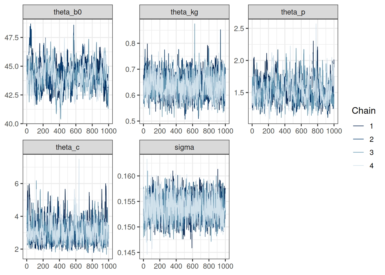
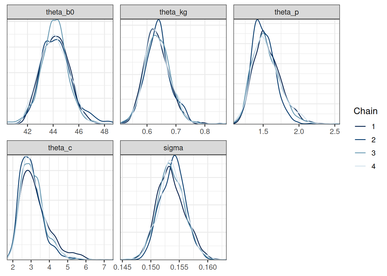
Let’s first look at the population level parameters:

cb_pop_params <- c("theta_b0", "theta_kg", "theta_p", "theta_c", "sigma")

mcmc_trace(post_df, pars = cb_pop_params)

mcmc_dens_overlay(post_df, pars = cb_pop_params)

mcmc_pairs(
  post_df, 
  pars = cb_pop_params,
  off_diag_args = list(size = 1, alpha = 0.1)
)

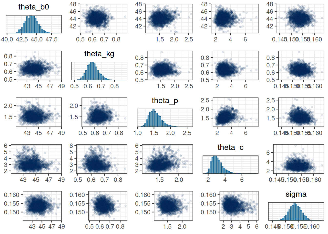
The trace plots look good. The chains seem to have converged and the pairs plot shows no strong correlations between the parameters. Let’s check the table:

post_sum <- post_df |>
  dplyr::select(theta_b0, theta_kg, theta_p, theta_c, omega_0, omega_g, omega_p, omega_c,
  cv_0, cv_g, cv_p, cv_c,
  sigma) |>
  summarize_draws() |>
  gt() |>
  fmt_number(decimals = 3)

Warning: Dropping 'draws_df' class as required metadata was removed.

post_sum

variable	mean	median	sd	mad	q5	q95	rhat	ess_bulk	ess_tail
theta_b0	44.142	44.118	1.093	1.090	42.411	45.949	1.003	198.908	390.883
theta_kg	0.636	0.634	0.042	0.041	0.570	0.711	1.000	1,093.102	1,749.378
theta_p	1.539	1.515	0.183	0.179	1.284	1.871	1.002	361.463	395.589
theta_c	3.098	2.984	0.678	0.607	2.234	4.366	1.001	552.128	669.150
omega_0	0.581	0.581	0.016	0.016	0.556	0.608	1.003	429.108	1,002.446
omega_g	1.043	1.040	0.063	0.062	0.943	1.149	1.004	664.633	1,063.643
omega_p	1.576	1.570	0.105	0.104	1.413	1.757	1.001	434.576	976.113
omega_c	1.569	1.565	0.150	0.153	1.326	1.822	1.001	638.934	941.209
cv_0	0.634	0.634	0.020	0.021	0.602	0.669	1.003	429.108	1,002.446
cv_g	1.409	1.396	0.140	0.136	1.197	1.655	1.004	664.633	1,063.643
cv_p	3.383	3.278	0.645	0.578	2.521	4.577	1.001	434.576	976.113
cv_c	3.415	3.254	0.930	0.838	2.192	5.165	1.001	638.934	941.209
sigma	0.154	0.154	0.002	0.002	0.150	0.158	1.000	1,258.184	2,273.384

We see similar estimated values as before for \(\theta_{b_{0}}\), \(\theta_{k_{g}}\) and \(\sigma\).

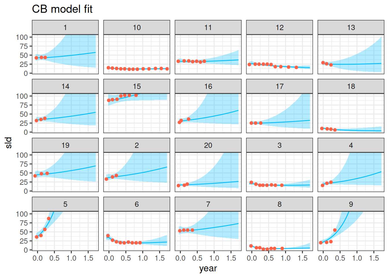
Observation vs model fit

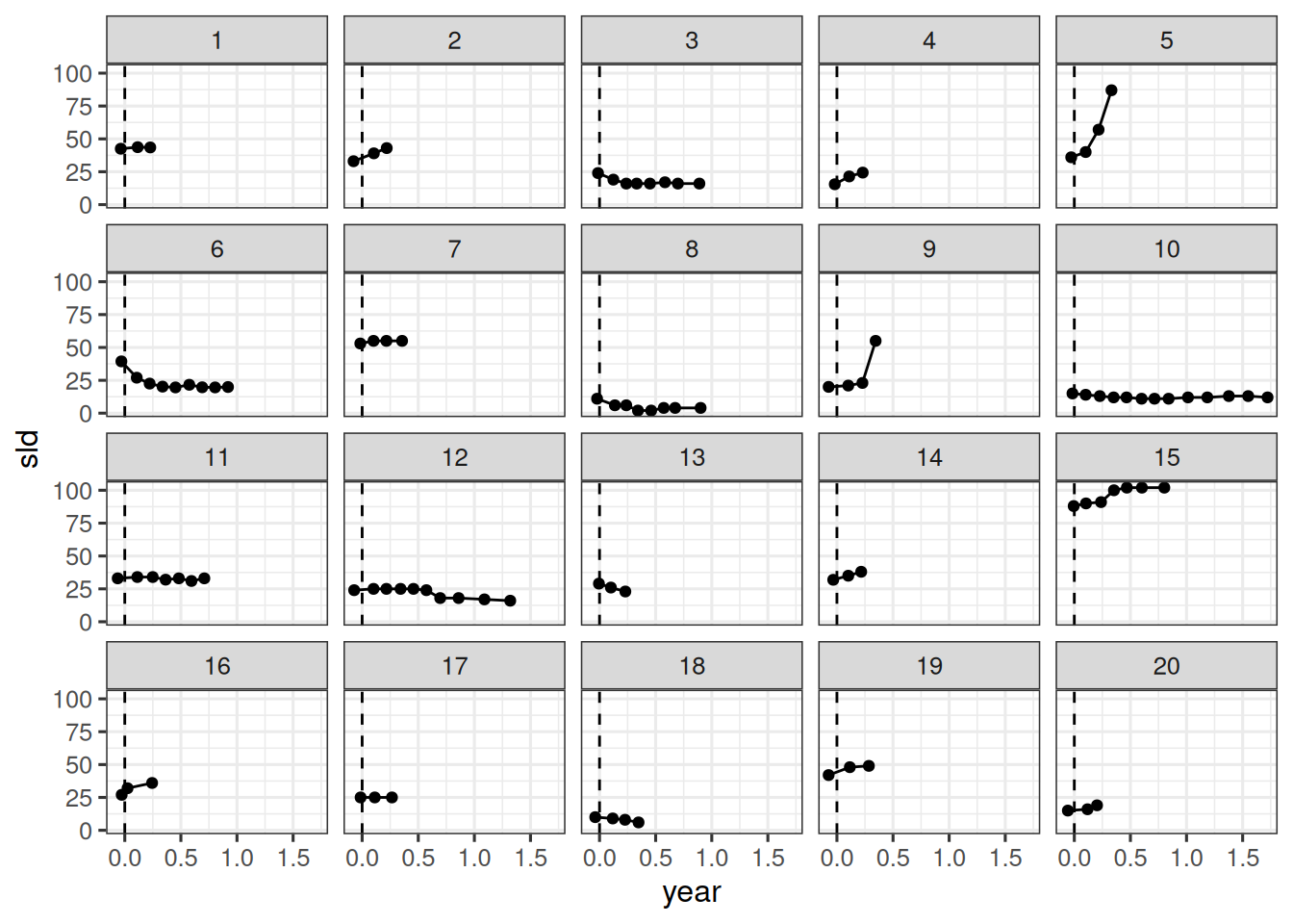
We can now compare the model fit to the observations. Let’s do this for the first 20 patients again:

pt_subset <- as.character(1:20)
df_subset <- df |> 
  filter(id %in% pt_subset)

df_sim_save_file <- here("session-tgi/cb3_sim_df.RData")
if (file.exists(df_sim_save_file)) {
  load(df_sim_save_file)
} else {
  df_sim <- df_subset |> 
    data_grid(
      id = pt_subset, 
      year = seq_range(year, 101)
    ) |>
    add_epred_draws(fit) |>
    median_qi()
  save(df_sim, file = df_sim_save_file)
}

df_sim |>
  ggplot(aes(x = year, y = sld)) +
  facet_wrap(~ id) +
  geom_ribbon(
    aes(y = .epred, ymin = .lower, ymax = .upper), 
    alpha = 0.3, 
    fill = "deepskyblue"
  ) +
  geom_line(aes(y = .epred), color = "deepskyblue") +
  geom_point(data = df_subset, color = "tomato") +
  coord_cartesian(ylim = range(df_subset$sld)) +
  scale_fill_brewer(palette = "Greys") +
  labs(title = "CB model fit")

Warning: Removed 1 row containing missing values or values outside the scale range
(`geom_line()`).

This also looks good. The model seems to capture the data well.

With jmpost

This model can also be fit with the jmpost package. The corresponding function is LongitudinalClaretBruno. The statistical model is specified in the vignette here.

Homework: Implement the generalized Claret-Bruno model with jmpost and compare the results with the brms implementation.